Overview

이번 과제에서는 label 없이 image representation을 학습하는 self-supervised learning과 SimCLR의 contrastive learning을 구현하고, 학습된 representation이 downstream image classification에 얼마나 유용한지 평가한다.

Supervised learning은 이미지와 사람이 붙인 class label의 관계를 학습한다. 반면 self-supervised learning은 data 자체에서 학습 신호를 만든다. SimCLR에서는 같은 이미지에 서로 다른 random augmentation을 적용해 두 view를 만들고, 이 둘을 positive pair로 취급한다. Model은 positive pair의 representation을 가깝게 만들고, batch 안의 다른 이미지에서 나온 view는 멀어지게 학습한다.

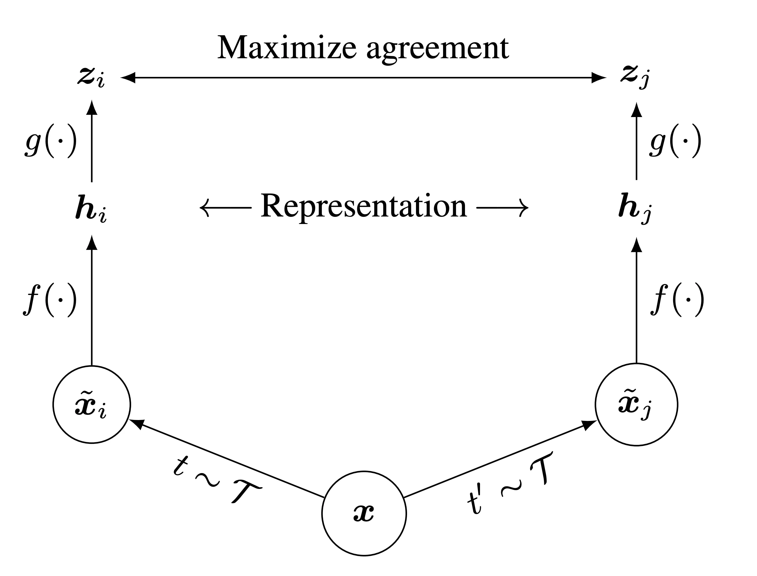
Notebook에 포함된 SimCLR 논문 Figure 2이다.

SimCLR의 전체 흐름은 다음과 같다.

$$x \xrightarrow{t,t'\sim\mathcal{T}} (\tilde{x}_i,\tilde{x}_j) \xrightarrow{f} (h_i,h_j) \xrightarrow{g} (z_i,z_j) \xrightarrow{\text{NT-Xent}} \mathcal{L}$$

• $x$는 원본 이미지
• $t$와 $t'$는 augmentation family $\mathcal{T}$에서 독립적으로 sampling한 transformation
• $\tilde{x}_i$와 $\tilde{x}_j$는 같은 원본에서 만든 두 augmented view
• $f$는 base encoder이며 downstream task에 사용할 representation $h$를 만듬
• $g$는 contrastive loss를 계산할 projection space로 옮기는 projection head
• $z=g(h)$는 NT-Xent loss가 직접 적용되는 vector

Pretraining이 끝나면 projection head $g$는 버리고 base encoder $f$가 만든 $h$를 downstream task에 사용한다. 즉 contrastive objective는 $z$에서 최적화하지만 최종적으로 얻고 싶은 것은 여러 task에 재사용할 수 있는 $h$이다.

이번 notebook은 CIFAR-10으로 오래 pretrain한 checkpoint를 불러온 뒤 50%의 training data로 1 epoch를 추가 학습한다. 이후 frozen representation에 대한 $k$NN 평가와 linear evaluation을 수행한다. 두 평가는 class label을 사용해 representation의 품질을 측정하지만, contrastive pretraining 자체는 class label을 loss에 사용하지 않는다.

핵심 아이디어

Self-supervised learning은 data에서 supervision을 만든다

Self-supervised learning의 핵심은 사람이 정답 label을 붙이지 않아도 data의 구조로부터 prediction target을 만드는 것이다. SimCLR에서 target은 class name이 아니라 어떤 두 view가 같은 원본 이미지에서 나왔는가이다.

좋은 image representation은 같은 semantic object의 여러 view를 비슷하게 표현하면서, 서로 다른 이미지는 구분할 수 있어야 한다. 이를 다음 두 성질로 나눠 생각할 수 있다.

• Invariance(불변성): crop, flip, color 변화가 있어도 같은 이미지의 핵심 의미는 유지한다.
• Discriminability(변별력): 다른 이미지에서 나온 representation은 구별할 수 있다.

Positive pair의 유사도만 높이도록 학습하면, 모든 입력을 동일한 vector로 매핑하는 것만으로도 objective를 만족할 수 있어 representation collapse가 발생할 수 있다. SimCLR는 batch 내의 다른 sample들을 negative로 사용해 서로 다른 sample의 representation은 멀어지도록 학습함으로써 이러한 collapse를 방지한다.

Data augmentation이 학습할 invariance를 정의

원본 이미지 $x$에 두 transformation을 독립적으로 적용한다.

$$\tilde{x}_i=t(x), \qquad \tilde{x}_j=t'(x), \qquad t,t'\sim\mathcal{T}$$

두 view의 pixel 값과 보이는 영역은 달라도 같은 원본에서 나왔으므로 positive pair이다. Model은 이 둘을 가깝게 만들어야 하므로 augmentation에 의해 바뀐 정보에는 둔감하고, 두 view에 공통으로 남아 있는 semantic information을 보존하도록 학습된다.

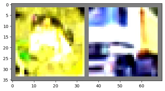
위 notebook 출력은 positive pair가 아니라 CIFAR-10 batch에서 가져온 서로 다른 두 sample에 training transform을 적용한 결과이다. 실제 CIFAR10Pair는 한 이미지에 같은 stochastic transform을 독립적으로 두 번 호출해 positive pair를 만든다.

Notebook의 training transform은 다음 연산을 조합한다.

1. 이미지를 무작위로 crop하고 $32\times32$로 resize
2. 확률 $0.5$로 horizontal flip을 적용
3. 확률 $0.8$로 brightness, contrast, saturation, hue를 바꾸는 color jitter를 적용
4. 확률 $0.2$로 grayscale image로 변환

Augmentation은 어떤 변화 전후를 같은 것으로 볼 것인지 정의하므로 contrastive prediction task 자체를 결정한다. 예를 들어 crop만 적용하면 같은 이미지에서 나온 patch들이 비슷한 color histogram을 공유해 model이 색 분포라는 shortcut으로 positive pair를 찾을 수 있다. SimCLR 논문은 random crop과 color distortion의 조합이 이런 shortcut을 줄이고 더 일반적인 representation을 만드는 데 특히 중요하다고 설명한다.

반대로 semantic class를 바꿀 정도로 강한 augmentation을 사용하면 실제로 다른 의미의 두 view를 positive pair로 묶게 된다. 따라서 augmentation은 downstream task에서 유지되어야 할 정보와 제거해도 되는 변화를 기준으로 설계해야 한다.

Base encoder와 projection head의 역할은 다르다

Base encoder $f$는 augmented view를 representation $h$로 변환한다.

$$h_i=f(\tilde{x}_i)$$

Projection head $g$는 $h_i$를 contrastive loss가 작동할 공간의 vector $z_i$로 바꾼다. SimCLR 원문은 hidden layer 하나와 ReLU를 가진 MLP를 사용한다.

$$z_i = g(h_i) = W^{(2)}\sigma\left(W^{(1)}h_i\right)$$

Projection head를 따로 두는 이유는 contrastive objective가 요구하는 invariance와 downstream task에 유용한 정보가 완전히 같지 않을 수 있기 때문이다. $z$는 augmentation 차이를 지우는 데 직접 최적화되므로 color나 orientation처럼 다른 task에서 필요할 수 있는 정보까지 잃을 수 있다. $g$가 loss에 필요한 변환을 담당하게 하면 그 앞의 $h$에는 더 넓은 정보를 남길 수 있다.

SimCLR 논문에서도 nonlinear projection head를 사용했을 때 그 앞의 representation $h$의 linear evaluation 성능이 좋아졌으며, downstream representation으로는 projection 이후의 $z$보다 projection 이전의 $h$가 더 우수했다. 따라서 pretraining 후에는 $g$를 버리고 $f$의 출력 $h$를 사용한다.

Cosine similarity는 방향의 일치를 비교한다

SimCLR는 두 projection vector의 normalized dot product, 즉 cosine similarity를 사용한다.

$$\operatorname{sim}(u,v) = \frac{u^\top v}{\lVert u\rVert_2\lVert v\rVert_2}$$

Vector norm을 제거하므로 score를 크게 만들기 위해 magnitude만 키우는 방향을 막고, 두 vector의 방향이 얼마나 일치하는지 비교한다. Positive pair의 similarity는 높이고 negative pair의 similarity는 낮추는 것이 목표이다.

NT-Xent loss

원본 image $N$개를 sampling하고 각 이미지에서 두 view를 만들면 한 batch에는 $2N$개의 augmented sample이 생긴다. Notebook에서는 첫 번째 view들을 $z_1,\ldots,z_N$, 두 번째 view들을 $z_{N+1},\ldots,z_{2N}$ 순서로 배치한다. 따라서 $z_k$의 positive는 $z_{k+N}$이다.

Anchor $i$와 positive $j$에 대한 NT-Xent loss는 다음과 같다.

$$\ell(i,j) = -\log \frac{ \exp\left(\operatorname{sim}(z_i,z_j)/\tau\right) }{ \displaystyle \sum_{k=1}^{2N} \mathbb{1}_{[k\neq i]} \exp\left(\operatorname{sim}(z_i,z_k)/\tau\right) }$$

기호의 의미는 다음과 같다.

• $z_i$는 기준이 되는 anchor
• $z_j$는 같은 원본 이미지에서 나온 positive
• $z_k$는 batch에 있는 모든 augmented sample
• $\mathbb{1}_{[k\neq i]}$는 anchor 자신을 denominator에서 제외
• $\tau$는 similarity logit의 scale을 조절하는 temperature

Denominator에는 positive 하나와 다른 이미지에서 만들어진 $2N-2$개의 negative가 들어간다. 이 식은 anchor $i$가 나머지 $2N-1$개 candidate 중 자신의 positive $j$를 맞히는 cross-entropy로 볼 수 있다. 유한한 logit에서 positive의 softmax probability는 $(0,1)$에 있고 $-\log p$는 양수이다. Positive similarity가 다른 모든 similarity보다 충분히 커지면 probability가 $1$에 가까워지고 loss는 $0$에 가까워진다.

Positive pair는 방향을 바꿔서도 각각 학습한다. Notebook의 전체 loss는 다음과 같다.

$$\mathcal{L} = \frac{1}{2N} \sum_{k=1}^{N} \left[ \ell(k,k+N) + \ell(k+N,k) \right]$$

각 view가 한 번씩 anchor가 되므로 한쪽 branch만 기준으로 학습하는 것보다 대칭적인 learning signal을 얻는다.

Temperature가 similarity 분포를 조절

NT-Xent는 cosine similarity를 $\tau$로 나눈 뒤 exponential을 취한다.

$$p_{i,j} = \frac{ \exp\left(\operatorname{sim}(z_i,z_j)/\tau\right) }{ \displaystyle \sum_{k\neq i} \exp\left(\operatorname{sim}(z_i,z_k)/\tau\right) }$$

$\tau$가 작으면 similarity 차이가 크게 확대되어 분포가 sharp해지고, anchor와 비슷한 hard negative에 gradient가 집중된다. $\tau$가 크면 candidate 사이의 차이가 완만해진다. 너무 작으면 일부 pair에만 gradient가 집중되고, 너무 크면 positive와 negative의 차이를 충분히 강조하지 못하므로 embedding normalization과 함께 적절한 값을 선택해야 한다. 이번 과제에서는 $\tau=0.5$를 사용한다.

구현

Data augmentation

Training transform은 같은 원본에서 모양과 색이 다른 두 view를 만들 수 있도록 네 가지 random augmentation을 순서대로 적용한다. ColorJitter는 먼저 객체로 만든 뒤 RandomApply로 감싸 전체 color 변환의 적용 확률을 $0.8$로 설정한다.

from torchvision import transforms
import random
import torch


def compute_train_transform(seed=123456):
    random.seed(seed)
    torch.random.manual_seed(seed)

    color_jitter = transforms.ColorJitter(
        brightness=0.4,
        contrast=0.4,
        saturation=0.4,
        hue=0.1,
    )

    train_transform = transforms.Compose([
        transforms.RandomResizedCrop(32),
        transforms.RandomHorizontalFlip(p=0.5),
        transforms.RandomApply([color_jitter], p=0.8),
        transforms.RandomGrayscale(p=0.2),
        transforms.ToTensor(),
        transforms.Normalize(
            [0.4914, 0.4822, 0.4465],
            [0.2023, 0.1994, 0.2010],
        ),
    ])
    return train_transform

CIFAR10Pair는 하나의 원본 img에 같은 transform 객체를 독립적으로 두 번 호출한다. Transform 내부의 random parameter가 호출할 때마다 새로 sampling되므로 x_i와 x_j는 같은 image에서 나왔지만 서로 다른 crop과 color를 가진 positive pair가 된다.

from PIL import Image
from torchvision.datasets import CIFAR10


class CIFAR10Pair(CIFAR10):
    def __getitem__(self, index):
        img, target = self.data[index], self.targets[index]
        img = Image.fromarray(img)

        x_i = None
        x_j = None

        if self.transform is not None:
            x_i = self.transform(img)
            x_j = self.transform(img)

        if self.target_transform is not None:
            target = self.target_transform(target)

        return x_i, x_j, target

Dataset은 target도 반환하지만 contrastive pretraining의 train()에서는 이를 loss 계산에 사용하지 않는다. Label은 이후 $k$NN과 linear evaluation에만 사용한다.

Base encoder와 projection head

Base encoder에는 ResNet-50을 사용한다. CIFAR-10 image가 $32\times32$로 작기 때문에 ImageNet용 첫 7×7, stride 2 convolution을 3×3, stride 1 convolution으로 바꾸고, 초기 max pooling과 마지막 classification layer는 제거한다. avgpool까지 통과한 feature를 flatten하면 sample마다 2048차원 representation $h$를 얻는다.

Projection head $g$는 2048 → 512 → 128 MLP이다. Encoder feature와 projection output을 모두 L2 normalize해서 반환하지만, NT-Xent loss에는 두 번째 반환값인 128차원 $z$를 사용한다.

import torch
import torch.nn as nn
import torch.nn.functional as F
from torchvision.models import resnet50


class Model(nn.Module):
    def __init__(self, feature_dim=128):
        super(Model, self).__init__()

        self.f = []
        for name, module in resnet50().named_children():
            if name == 'conv1':
                module = nn.Conv2d(
                    3,
                    64,
                    kernel_size=3,
                    stride=1,
                    padding=1,
                    bias=False,
                )
            if (
                not isinstance(module, nn.Linear)
                and not isinstance(module, nn.MaxPool2d)
            ):
                self.f.append(module)

        # encoder
        self.f = nn.Sequential(*self.f)

        # projection head
        self.g = nn.Sequential(
            nn.Linear(2048, 512, bias=False),
            nn.BatchNorm1d(512),
            nn.ReLU(inplace=True),
            nn.Linear(512, feature_dim, bias=True),
        )

    def forward(self, x):
        x = self.f(x)
        feature = torch.flatten(x, start_dim=1)
        out = self.g(feature)
        return F.normalize(feature, dim=-1), F.normalize(out, dim=-1)

주요 tensor shape은 다음과 같다.

값	의미	Shape
x_i, x_j	두 augmented view batch	$(N,3,32,32)$
feature	L2-normalized encoder representation$h$	$(N,2048)$
out	L2-normalized projection$z$	$(N,128)$
out_left, out_right	두 branch의 projection batch	각각$(N,D)$
out in loss	두 branch를 합친 projection	$(2N,D)$
sim_matrix	모든 augmented sample 사이의 cosine similarity	$(2N,2N)$

Normalized dot product

두 vector의 similarity는 dot product를 norm의 곱으로 나누어 계산한다.

def sim(z_i, z_j):
    norm_dot_product = torch.sum(z_i * z_j) / (
        torch.linalg.norm(z_i) * torch.linalg.norm(z_j)
    )
    return norm_dot_product

Model이 반환하는 $z$는 이미 L2 normalize되어 있으므로 정상적인 forward path에서는 이 값이 단순 dot product와 같다. 함수를 독립적으로 test할 때는 입력이 normalize되어 있다는 보장이 없으므로 위처럼 norm으로 직접 나눈다.

NT-Xent loss의 naive 구현

Naive 구현은 positive pair마다 두 방향의 loss를 각각 계산한다. out_left[k]를 anchor로 할 때는 자기 자신인 index $k$만 denominator에서 제외하고, out_right[k]를 anchor로 할 때는 index $k+N$을 제외한다.

def simclr_loss_naive(out_left, out_right, tau):
    N = out_left.shape[0]  # total number of training examples

    # Concatenate out_left and out_right into a 2*N x D tensor.
    out = torch.cat([out_left, out_right], dim=0)  # [2*N, D]

    total_loss = 0
    for k in range(N):  # loop through each positive pair (k, k+N)
        z_k, z_k_N = out[k], out[k + N]

        numerator = torch.exp(sim(z_k, z_k_N) / tau)
        denominator = 0
        for j in range(2 * N):
            if j == k:
                continue
            denominator += torch.exp(sim(z_k, out[j]) / tau)
        loss_k = -torch.log(numerator / denominator)

        numerator_reverse = torch.exp(sim(z_k_N, z_k) / tau)
        denominator_reverse = 0
        for j in range(2 * N):
            if j == k + N:
                continue

            denominator_reverse += torch.exp(
                sim(z_k_N, out[j]) / tau
            )

        loss_k_N = -torch.log(
            numerator_reverse / denominator_reverse
        )

        # 두 방향 loss 누적
        total_loss += loss_k + loss_k_N

    # In the end, we need to divide the total loss by 2N,
    # the number of samples in the batch.
    total_loss = total_loss / (2 * N)
    return total_loss

한 positive pair $(k,k+N)$에 대해 loss_k와 loss_k_N을 모두 더한다. 이는 notebook에 적어둔 것처럼 모든 sample을 한 번씩 anchor로 사용한 뒤 $2N$으로 평균내는 과정이다.

Naive 구현은 각 anchor마다 나머지 $2N-1$개 sample을 순회한다. 필요한 pair 비교 수는 어차피 $O(N^2)$이지만, 작은 tensor 연산을 반복 호출하므로 GPU 병렬성을 충분히 사용하지 못한다.

Positive pair를 한 번에 계산하기

같은 row의 out_left[k]와 out_right[k]만 곱하고 feature dimension을 합하면 $N$개 positive pair의 dot product를 한 번에 얻는다. keepdim=True를 사용해 결과 shape을 $(N,1)$로 유지한다.

def sim_positive_pairs(out_left, out_right):
    dot_product = torch.sum(
        out_left * out_right,
        dim=1,
        keepdim=True,
    )  # (N, 1)

    norm = (
        torch.linalg.norm(out_left, dim=1, keepdim=True)
        * torch.linalg.norm(out_right, dim=1, keepdim=True)
    )  # (N, 1)

    pos_pairs = dot_product / norm
    return pos_pairs

Sanity input에서 계산한 positive similarity는 0.7820, 0.9256이었다. 같은 연산을 row별 loop 없이 수행하면서도 각 row끼리만 pair가 되도록 feature dimension인 dim=1을 합하는 것이 포인트다.

전체 similarity matrix

두 branch를 이어 붙인 out을 row별로 normalize한 뒤 자기 자신의 transpose와 행렬곱하면 모든 pair의 cosine similarity를 얻는다.

def compute_sim_matrix(out):
    # out.shape = (2N, D)
    norm = torch.linalg.norm(out, dim=1, keepdim=True)  # (2N, 1)
    norm_out = out / norm  # (2N, D)

    sim_matrix = norm_out @ norm_out.T  # (2N, 2N)
    return sim_matrix

이를 수식으로 쓰면 다음과 같다. $Z$는 각 row가 하나의 projection인 $(2N,D)$ 행렬이고, $\bar Z$는 row normalization을 적용한 행렬이다.

$$\bar Z_i = \frac{Z_i}{\lVert Z_i\rVert_2}, \qquad S = \bar Z\bar Z^T$$

$S_{ij}$는 $z_i$와 $z_j$의 cosine similarity이다. 대각 원소 $S_{ii}=1$은 자기 자신과의 similarity이므로 denominator에서 제거해야 한다.

NT-Xent loss의 vectorized 구현

Vectorized 구현은 similarity matrix를 exponential로 바꾼 뒤, identity matrix를 이용한 mask로 대각 원소를 한 번에 제거한다.

def simclr_loss_vectorized(
    out_left,
    out_right,
    tau,
    device='cuda',
):
    N = out_left.shape[0]

    # Concatenate out_left and out_right into a 2*N x D tensor.
    out = torch.cat([out_left, out_right], dim=0)  # [2*N, D]

    # Compute similarity matrix between all pairs of augmented examples.
    sim_matrix = compute_sim_matrix(out)  # [2*N, 2*N]

    exponential = torch.exp(sim_matrix / tau)

    # This binary mask zeros out terms where k=i.
    mask = (
        torch.ones_like(exponential, device=device)
        - torch.eye(2 * N, device=device)
    ).to(device).bool()

    # We apply the binary mask.
    exponential = exponential.masked_select(mask).view(
        2 * N,
        -1,
    )  # [2*N, 2*N-1]

    denominator = torch.sum(
        exponential,
        dim=1,
        keepdim=True,
    )  # (2N, 1)

    pos_sim = torch.cat([
        torch.diag(sim_matrix, diagonal=N),
        torch.diag(sim_matrix, diagonal=-N),
    ]).unsqueeze(1)

    numerator = torch.exp(pos_sim / tau)
    loss = -torch.log(numerator / denominator).mean()

    return loss

Positive 위치가 diagonal offset $\pm N$에 놓이는 이유는 concatenation 순서 때문이다.

$$Z = [z^{L}_0,\ldots,z^{L}_{N-1},z^{R}_0,\ldots,z^{R}_{N-1}]^T$$

• diagonal=N은 $S_{k,k+N}$을 가져온다.
• diagonal=-N은 $S_{k+N,k}$을 가져온다.
• 두 vector를 연결하면 denominator의 row 순서인 left anchor $N$개, right anchor $N$개와 정확히 맞는다.

masked_select는 대각 원소를 제외한 각 row의 $2N-1$개 값을 모은다. 그 합이 denominator이며, pos_sim에서 만든 positive score가 numerator이다. 마지막 .mean()은 $2N$개 anchor loss의 평균을 계산한다.

Contrastive pretraining loop

각 minibatch는 (x_i, x_j, target)을 반환한다. 두 view를 같은 model에 통과시키고 projection output만 가져와 vectorized NT-Xent loss를 계산한다.

def train(
    model,
    data_loader,
    train_optimizer,
    epoch,
    epochs,
    batch_size=32,
    temperature=0.5,
    device='cuda',
):
    model.train()
    total_loss, total_num = 0.0, 0
    train_bar = tqdm(data_loader)

    for data_pair in train_bar:
        x_i, x_j, target = data_pair
        x_i, x_j = x_i.to(device), x_j.to(device)

        _, out_left = model(x_i)
        _, out_right = model(x_j)
        loss = simclr_loss_vectorized(
            out_left,
            out_right,
            tau=temperature,
            device=device,
        )

        train_optimizer.zero_grad()
        loss.backward()
        train_optimizer.step()

        total_num += batch_size
        total_loss += loss.item() * batch_size
        train_bar.set_description(
            'Train Epoch: [{}/{}] Loss: {:.4f}'.format(
                epoch,
                epochs,
                total_loss / total_num,
            )
        )

    return total_loss / total_num

target을 읽기는 하지만 loss에는 전달하지 않는다. 두 augmentation이 같은 dataset index에서 나왔다는 사실이 supervision 역할을 한다. 첫 번째 반환값 $h$ 대신 두 번째 반환값 $z$를 loss에 사용하는 것도 중요하다.

이번 실행에서는 drop_last=True이므로 모든 batch의 크기가 설정값과 같아 total_num += batch_size가 맞다. 일반적인 loader에서 마지막 batch가 더 작을 수 있다면 current_batch_size = x_i.size(0)을 사용해 loss 평균을 누적하는 편이 안전하다.

Linear classifier와 evaluation protocol

Downstream classifier는 projection head를 사용하지 않는다. Encoder $f$가 만든 2048차원 feature에 10-class linear layer를 바로 연결한다.

class Classifier(nn.Module):
    def __init__(self, num_class):
        super(Classifier, self).__init__()

        # Encoder.
        self.f = Model().f

        # Classifier.
        self.fc = nn.Linear(2048, num_class, bias=True)

    def forward(self, x):
        x = self.f(x)
        feature = torch.flatten(x, start_dim=1)
        out = self.fc(feature)
        return out

Random baseline과 SimCLR checkpoint 실험 모두 다음 코드로 encoder parameter의 gradient를 끄고 linear layer만 optimizer에 전달한다.

for param in model.f.parameters():
    param.requires_grad = False

optimizer = optim.Adam(
    model.fc.parameters(),
    lr=1e-3,
    weight_decay=1e-6,
)

ResNet-50 전체 parameter 수는 약 23.52M이지만 이 단계에서 gradient로 갱신되는 parameter는 마지막 layer의 weight와 bias뿐이다.

$$2048\times10+10=20{,}490$$

따라서 이 실험은 encoder 전체를 labeled data로 fine-tune하는 방식이 아닌 고정된 representation이 linear boundary만으로 class를 얼마나 잘 나누는지 확인하는 linear evaluation이다.

실험 결과

구현 sanity check

Notebook에 저장된 test output은 naive 구현과 vectorized 구현이 제공된 정답에 맞는지 확인한다.

검사 대상	결과
Data augmentation maximum error	0
sim maximum error	$3.81097\times10^{-8}$ 이하
Naive loss maximum error	$5.65617\times10^{-8}$ 이하
Positive pair similarity maximum error	$3.81097\times10^{-8}$
Similarity matrix	Test passed
Vectorized loss maximum error	$5.65617\times10^{-8}$ 이하

Pretrained model 추가 학습

Notebook은 CIFAR-10으로 약 18시간 동안 pretrain한 SimCLR checkpoint를 제공한다. 이 checkpoint를 불러온 뒤 CIFAR-10 training set의 50%를 사용해 1 epoch를 추가 학습한다. 따라서 아래 결과는 random initialization에서 1 epoch만 학습한 결과가 아니다.

선택한 sample은 25,000개이지만 batch_size=64, drop_last=True이므로 이 epoch에서 실제로 사용된 sample은 $390\times64=24{,}960$개이다.

설정	값
추가 pretraining data	CIFAR-10 training set의 50%
Epoch	1
Batch size	64
Projection dimension	128
Temperature$\tau$	0.5
Optimizer	Adam
Learning rate	$10^{-3}$
Weight decay	$10^{-6}$
$k$NN의 $k$	200
Model 규모	24.62M parameters, 1.31G FLOPs

추가 pretraining과 frozen feature-space $k$NN 평가 결과는 다음과 같다.

지표	결과
추가 pretraining loss	3.2578
$k$NN Acc@1	83.43%
$k$NN Acc@5	99.31%

Pretraining loss는 NT-Xent objective의 값이며 classification accuracy와 직접 같은 척도가 아니다. $k$NN 평가는 encoder가 만든 normalized representation을 사용해 training feature bank에서 가까운 sample을 찾고 test image의 class를 예측한다. 별도의 parametric classifier를 학습하지 않아도 Acc@1이 83.43%라는 것은 같은 class의 이미지가 feature space에서 상당히 잘 모였음을 보여준다.

Acc@5는 정답 class가 상위 5개 prediction 안에 들어가는 비율이다. CIFAR-10은 class가 10개뿐이므로 Acc@5 99.31%는 representation이 정답 후보를 거의 항상 상위 절반 안에 둔다는 뜻이다. 다만 class 절반을 정답으로 허용하는 지표이므로 이 실험에서는 Acc@1이 더 구분력 있는 수치이다.

Frozen encoder linear evaluation

Notebook은 projection head를 제거하고 encoder $f$의 2048차원 출력 위에 10-class linear layer를 붙인다. 여기서 notebook의 섹션 이름은 finetune이라고 되어 있지만, 실제 실행 코드는 두 비교군 모두 encoder를 freeze하고 마지막 linear layer만 학습한다.

두 실험에서 공통으로 다음 설정이 적용된다.

• model.f의 모든 parameter에 대해 gradient를 비활성화한다.
• Optimizer에는 마지막 linear layer의 parameter만 전달한다.
• CIFAR-10 labeled training data의 10%로 linear layer를 10 epoch 학습한다.
• Encoder의 learnable weight는 학습 내내 바뀌지 않는다.

다만 제공된 train_val()은 training 시점에 전체 classifier를 train mode로 전환한다. requires_grad=False는 parameter gradient만 막으므로 encoder 안의 BatchNorm running mean과 variance는 바뀔 수 있다. 엄밀하게 모든 encoder state를 고정한 linear evaluation이라면 classifier를 학습할 때도 model.f.eval()을 유지해야 한다.

따라서 비교 대상은 다음과 같다.

비교군	Frozen encoder의 상태	학습되는 parameter
Baseline	Random initialization	마지막 linear layer만 학습
SSL pretrained	SimCLR pretrained weight	마지막 linear layer만 학습

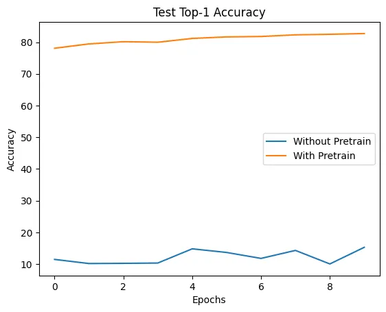
Notebook 그래프의 x축은 list index라 $0$부터 $9$까지 표시되지만, 실제로는 epoch 1부터 10까지의 결과이다.

Epoch	Random encoder Top-1	SimCLR encoder Top-1
1	11.48%	78.09%
2	10.18%	79.46%
3	10.24%	80.16%
4	10.34%	79.99%
5	14.82%	81.19%
6	13.67%	81.67%
7	11.80%	81.80%
8	14.32%	82.33%
9	10.05%	82.49%
10	15.30%	82.73%

Best top-1 accuracy는 다음과 같다.

평가	Best top-1 accuracy
Random frozen encoder + linear probe	15.30%
SSL pretrained frozen encoder + linear probe	82.73%
절대 향상 폭	+67.43%p

마지막 epoch의 Top-5 accuracy는 random encoder가 58.28%, SimCLR encoder가 98.90%였다. 전체 epoch에서 가장 높은 Top-5 accuracy는 각각 59.70%, 98.97%였다.

향상 폭은 두 accuracy의 차이이다.

$$82.73\%-15.30\%=67.43\text{ percentage points}$$

Random frozen encoder의 출력은 class를 구분하도록 학습된 적이 없으므로 linear layer 하나만으로는 CIFAR-10 class를 잘 분리하지 못한다. Best top-1 accuracy가 15.30%로 random guess 10%보다 조금 높은 수준에 머문 이유이다.

반면 SimCLR pretrained encoder는 class label을 보지 않고도 augmentation에 invariant하면서 이미지를 구분하는 feature를 학습했다. Encoder weight에 gradient update를 적용하지 않고 linear decision boundary만 학습했는데도 82.73%를 기록했다. 이는 downstream label을 사용하기 전에 이미 representation $h$ 안에 semantic class structure가 상당 부분 형성되어 있음을 보여준다.

이 결과를 SSL model과 end-to-end supervised model의 성능 차이로 해석하면 안 된다. Baseline에서도 encoder를 freeze했기 때문에 random encoder는 supervised signal로 feature를 학습할 기회가 없었다. 이 실험이 직접 측정하는 것은 두 frozen representation의 linear separability이며, +67.43%p는 pretraining으로 만들어진 representation quality의 차이를 보여준다.

추가 개념들

$k$NN evaluation과 linear evaluation의 차이

두 평가 모두 encoder를 바꾸지 않고 representation을 검사하지만 측정 방식은 다르다.

평가	예측 방식	추가 학습
$k$NN evaluation	Feature space에서 가까운 labeled sample의 class로 예측	없음
Linear evaluation	Frozen feature 위에 linear classifier를 학습	Linear layer만 학습

$k$NN은 local neighborhood가 class별로 잘 형성되었는지 확인한다. Linear evaluation은 전체 feature space에서 class가 linear boundary로 얼마나 잘 나뉘는지 확인한다. 따라서 두 수치는 representation의 서로 다른 기하학적 성질을 본다.

이번 notebook에서 $k$NN은 full training memory set과 $k=200$을 사용하지만, linear probe는 labeled training data의 10%만 사용한다. 평가 protocol이 다르므로 83.43%와 82.73%를 단순히 classifier 우열로 비교하기보다는 각각의 조건 안에서 해석해야 한다.

Linear evaluation은 full fine-tuning이 아니다

Linear evaluation에서는 다음 관계가 유지된다.

$$h=f(x), \qquad \hat{y}=W_{\mathrm{linear}}h+b$$

학습 중 갱신되는 것은 $W_{\mathrm{linear}}$와 $b$뿐이며 $f$의 parameter는 고정된다. 이 protocol은 downstream label이 encoder representation을 바꾸지 못하게 하므로 pretraining이 만든 feature를 직접 평가하기 좋다.

이번 코드에서는 encoder parameter의 gradient는 고정되지만 training mode의 BatchNorm running statistics가 갱신될 수 있다. Strict linear evaluation을 재현하려면 encoder를 eval mode로 유지해 parameter와 buffer를 모두 고정해야 한다.

반면 full fine-tuning은 encoder와 classifier를 함께 업데이트한다. Full fine-tuning은 downstream 성능을 더 높일 수 있지만 label이 representation 자체를 바꾸므로, pretraining 직후의 feature quality만 분리해 보기는 어렵다. 따라서 notebook에서 사용하는 표현은 동작 기준으로는 finetuning보다 linear probe 또는 linear evaluation이 더 정확하다고 생각한다.

Self-supervised learning을 통해 유용한 representation이 학습되었는지를, encoder를 고정한 뒤 마지막 linear classifier만 학습해 평가하는 실험이다.
이 실험은 representation의 품질을 확인하는 데 목적이 있으며, self-supervised learning이 supervised learning보다 우수하다는 결론을 직접적으로 내리기 위한 실험은 아니다.

Contrastive pretraining은 label-free이지만 평가는 label을 사용한다

SimCLR pretraining에서는 CIFAR-10 class label이 NT-Xent loss에 들어가지 않는다. Positive 여부는 class가 아니라 같은 원본에서 나온 두 augmentation인지로 결정된다. 그러나 $k$NN accuracy를 계산하려면 memory sample의 label이 필요하고, linear classifier를 학습할 때도 labeled subset이 필요하다.

즉 이 실험에서 label-free인 부분은 representation pretraining이다. Downstream evaluation까지 label이 전혀 없는 것은 아니다. Self-supervised learning의 이점은 대량의 unlabeled data로 encoder를 먼저 학습하고, 이후 상대적으로 적은 labeled data로 task를 해결할 수 있다는 데 있다.

Batch size가 negative의 수를 결정한다

SimCLR는 별도 memory bank 없이 현재 minibatch의 다른 sample을 negative로 사용한다. 원본 이미지가 $N$개이면 augmented sample은 $2N$개이고, 한 anchor에는 positive 하나와 $2N-2$개의 negative가 존재한다.

$$\text{negatives per anchor}=2N-2$$

Batch가 커지면 한 update에서 비교할 negative가 많아진다. SimCLR 논문은 큰 batch와 긴 training이 contrastive learning의 수렴과 representation 성능에 도움이 된다고 보고한다. 다만 batch를 키우면 memory와 compute 비용도 증가하므로 실제 구현에서는 distributed training, memory bank, queue 같은 다른 설계가 필요할 수 있다.

Cross-entropy 형태로 구현하면 더 안정적이다

과제 구현은 exp, division, log를 차례로 계산한다. 수식을 그대로 확인하기에는 좋지만, $\tau$가 작거나 logit이 크면 exponential이 overflow할 수 있다. 대각 원소를 -inf로 mask한 logits와 positive index를 만들고 cross_entropy를 사용하면 내부의 logsumexp를 통해 같은 loss를 더 안정적으로 계산할 수 있다.

def simclr_loss_stable(out_left, out_right, tau):
    out = torch.cat([out_left, out_right], dim=0)
    out = F.normalize(out, dim=1)

    logits = out @ out.T / tau
    logits.fill_diagonal_(float('-inf'))

    N = out_left.shape[0]
    targets = (
        torch.arange(2 * N, device=out.device) + N
    ) % (2 * N)

    return F.cross_entropy(logits, targets)

targets[k]=k+N이고 targets[k+N]=k이므로 notebook의 양방향 positive mapping과 같다. 이 구현도 $(2N,2N)$ similarity matrix를 저장하므로 시간과 memory complexity 자체는 $O(N^2)$이다. Vectorization은 비교 횟수를 줄이기보다 같은 연산을 GPU가 병렬로 처리하게 만든다.

Batch negative는 semantic negative와 같지 않다

SimCLR는 class label을 보지 않으므로 서로 다른 원본 이미지에서 나온 view를 모두 negative로 취급한다. 두 원본이 모두 고양이 이미지여도 instance가 다르면 NT-Xent에서는 negative가 된다. SimCLR의 pretext task는 class-level classification이 아니라 각 원본 instance를 다른 instance와 구분하는 instance discrimination에 가깝다.

이런 pair는 semantic 관점에서는 false negative일 수 있다. 그럼에도 강한 augmentation으로 같은 instance의 여러 변형을 묶고 많은 data에서 반복 학습하면, encoder는 개별 pixel을 외우기보다 재사용 가능한 visual feature를 형성할 수 있다. 다만 false negative가 지나치게 많거나 semantic class가 매우 적은 dataset에서는 negative 구성 방식이 representation 학습에 영향을 줄 수 있다.

Contrastive task accuracy와 representation quality는 같지 않다

Positive pair를 맞히는 pretext task가 쉬워졌다고 downstream representation이 반드시 좋아지는 것은 아니다. SimCLR 논문에서는 단일 augmentation만 사용했을 때 contrastive task 자체는 거의 완벽하게 풀 수 있어도 linear evaluation 성능은 낮았다. Model이 semantic feature 대신 color histogram 같은 shortcut을 사용할 수 있기 때문이다.

따라서 pretraining loss나 contrastive accuracy만으로 성공을 판단하면 안 된다. Frozen $k$NN, linear evaluation, transfer learning처럼 downstream utility를 직접 확인해야 한다.

Projection space $z$와 representation space $h$를 구분해야 한다

Contrastive loss가 적용되는 $z$와 downstream에 사용하는 $h$는 목적이 다르다.

$$h=f(\tilde{x}), \qquad z=g(h)$$

$z$는 positive pair를 식별하는 objective에 특화된 공간이다. $h$는 projection head가 제거된 뒤 다른 task에 전달되는 representation이다. 논문은 nonlinear $g$가 contrastive objective에 필요한 정보 손실을 맡도록 함으로써 $h$가 더 풍부한 정보를 유지할 수 있다고 해석한다. 그래서 loss를 계산한 layer를 그대로 downstream feature로 쓰는 것이 항상 최선은 아니다.

구현에서 확인한 주의점

항목	현재 구현	더 안전한 방법
Zero norm	Norm으로 바로 나누므로 zero vector에서NaN 가능	F.normalize(..., eps=...) 또는 denominator clamp 사용
Device	Loss 함수의device='cuda'가 입력과 분리됨	device = out.device로 tensor에서 device를 얻음
마지막 batch	total_num += batch_size로 고정 크기 가정	x_i.size(0)으로 실제 batch size 사용
BatchNorm	Encoder parameter만 freeze하고 train mode 사용	Linear probe 중model.f.eval() 유지
Checkpoint	strict=False가 missing key를 숨길 수 있음	반환된 missing·unexpected key를 확인
DataLoader	Colab에서num_workers=16 경고 발생	Runtime 자원에 맞춰 worker 수를 낮춤

Augmentation 시각화에서는 normalized image를 img / 2 + 0.5로 되돌렸지만, 실제 transform은 CIFAR-10 channel별 mean과 standard deviation을 사용한다. 이 차이 때문에 notebook에 $[-0.433,1.877]$ 범위의 clipping warning이 남았다. 위 그림은 augmentation의 대략적인 모습만 확인하는 용도이며, 정확한 색을 복원하려면 channel별로 img * std + mean을 적용해야 한다.

실험 수치를 해석할 때의 주의점

Notebook은 매 epoch test_loader를 평가하고 그중 가장 높은 test accuracy를 best score로 기록한다. 엄밀한 model selection이라면 validation set으로 epoch와 hyperparameter를 선택한 뒤 test set은 마지막에 한 번만 사용하는 편이 바람직하다. 여러 epoch의 test 결과 중 최댓값을 선택하면 test set에 간접적으로 맞춰져 성능이 다소 낙관적으로 보일 수 있다.

또한 제공된 checkpoint가 이미 CIFAR-10에서 장시간 pretrain되어 있으므로 1 epoch 추가 학습 결과만 보고 SimCLR가 한 번의 epoch로 83.43%에 도달했다고 해석해서는 안 된다. 이번 실행은 pretrained representation을 이어 학습하고 assignment implementation이 정상적으로 연결되는지 확인한 실험이다.

원 논문과 이번 과제의 범위 차이

SimCLR 원 논문은 주로 ImageNet과 ResNet-50을 사용하고, random crop/color distortion/Gaussian blur를 조합한다. 대규모 batch와 긴 pretraining, nonlinear projection head, normalized embedding과 temperature의 효과를 체계적으로 ablation한다.

이번 과제는 CIFAR-10의 $32\times32$ image를 사용하고, 제공된 checkpoint를 짧게 이어 학습한 뒤 $k$NN과 linear probe로 representation을 평가한다. 따라서 논문의 대규모 ImageNet 결과를 재현하는 실험이라기보다 SimCLR의 핵심 구성 요소와 evaluation protocol을 작은 환경에서 직접 확인하는 과제이다.

참고 자료

• Ting Chen, Simon Kornblith, Mohammad Norouzi, Geoffrey Hinton, A Simple Framework for Contrastive Learning of Visual Representations, ICML 2020