Overview

이번 과제에서는 Denoising Diffusion Probabilistic Model(DDPM)의 핵심 구성요소를 구현하고, noisy image를 점진적으로 denoise하여 이미지를 생성하는 과정을 배운다.

DDPM은 데이터 분포에서 바로 샘플을 생성하는 대신, 먼저 실제 이미지에 Gaussian noise를 점진적으로 추가하는 Forward Diffusion을 정의하고, 반대로 노이즈에서 이미지를 복원하는 Reverse Diffusion을 학습한다. Forward process 자체는 고정된 noise schedule에 의해 결정되며, 실제로 학습되는 부분은 각 timestep에서 noisy image를 보고 노이즈 또는 원본 이미지를 예측하는 denoising model이다. 이 denoising model로 U-Net을 사용한다.

핵심 아이디어

DDPM의 전체 흐름은 다음과 같다.

$$x_0 \xrightarrow{q(x_t \mid x_0)} x_t \xrightarrow{\epsilon_\theta(x_t,t)} \hat{\epsilon} \xrightarrow{\text{Reverse Sampling}} x_{t-1} \xrightarrow{\cdots} x_0$$

• $x_0$는 원본 이미지
• $x_t$는 timestep $t$에서 노이즈가 추가된 이미지
• $q(x_t \mid x_0)$는 Forward Diffusion
• $\epsilon_\theta$는 U-Net 기반 denoising model
• $t$는 현재 noise level을 나타내는 timestep
• $c$는 text embedding과 같은 조건(condition)
• Reverse Sampling은 model prediction을 이용해 $x_t$에서 $x_{t-1}$을 샘플링하는 과정

Forward Diffusion에서는 original image와 Gaussian noise를 이용해 임의의 timestep에 해당하는 noisy image를 직접 생성한다.

$$q(x_t \mid x_0) \sim \mathcal{N} \left( x_t; \sqrt{\bar{\alpha}_t}x_0, (1-\bar{\alpha}_t)I \right)$$

여기서 noise는 다음 분포에서 샘플링한다.

$$\epsilon \sim \mathcal{N}(0,I)$$

이번 구현의 기본 objective는 pred_noise이며, U-Net은 $x_t$와 timestep $t$, condition $c$를 입력받아 Forward Diffusion에서 실제로 사용된 noise를 예측하도록 학습된다.

$$\hat{\epsilon} = \epsilon_\theta(x_t,t)$$

Noise Prediction objective는 실제 noise와 predicted noise 사이의 Mean Squared Error(MSE)를 최소화한다.

$$\mathbb{E}_{t,x_0,\epsilon} \left[ \left\| \epsilon - \epsilon_\theta \left( \sqrt{\bar{\alpha}_t}x_0 + \sqrt{1-\bar{\alpha}_t}\epsilon, t \right) \right\|^2 \right]$$

학습이 끝난 뒤 image generation은 Gaussian noise에서 시작한다. 각 timestep마다 U-Net prediction을 이용해 $x_0$를 추정하고, 사후분포(posterior distribution)를 계산한 뒤 $x_{t-1}$을 샘플링한다. 이 과정을 모든 timestep에 대해 반복하면서 노이즈를 점차 제거한다.

$$x_T \rightarrow x_{T-1} \rightarrow x_{T-2} \rightarrow \cdots \rightarrow x_0$$

U-Net은 이 Reverse Diffusion 과정에서 핵심 denoising model 역할을 한다. Downsampling 경로에서는 공간 해상도(spatial resolution)를 줄이면서 high-level feature를 추출하고, Upsampling 경로에서는 해상도(resolution)를 복원한다. Skip Connection을 통해 Downsampling 과정에서 보존한 세밀한 공간 정보를 Upsampling 단계에 전달한다.

이번 과제에서는 Conditional Generation을 위해 Classifier-Free Guidance(CFG)도 구현한다. 학습 중 일정 확률로 condition을 제거하여 하나의 U-Net이 Conditional Prediction과 Unconditional Prediction을 모두 학습하도록 한다.

샘플링시에는 같은 $x_t$에 대해 두 prediction을 계산하고 그 차이를 증폭하여 condition의 영향을 강화한다.

$$\epsilon_\theta(x_t,t,c) \leftarrow (w+1)\epsilon_\theta(x_t,t,c) - w\epsilon_\theta(x_t,t,\phi)$$

동일한 식은 다음처럼 표현할 수 있다.

$$\epsilon_\theta(x_t,t,c) + w \left( \epsilon_\theta(x_t,t,c) - \epsilon_\theta(x_t,t,\phi) \right)$$

따라서 guidance scale $w$가 커질수록 Conditional Prediction과 Unconditional Prediction의 차이가 더 강하게 반영되어 주어진 condition을 더 충실하게 따르는 generation을 만들 수 있다.

이 노트북에서는 직접 긴 시간 동안 모델을 학습하는 대신 Emoji 데이터셋으로 사전에 학습된 체크포인트를 불러와 샘플링에 사용한다. 구현 대상은 Forward Diffusion의 q_sample, DDPM training loss인 p_losses, Reverse Diffusion 한 step을 수행하는 p_sample, U-Net의 Downsampling/Upsampling 및 Skip Connection, 그리고 Classifier-Free Guidance이다.

구현

q_sample

함수 q_sample은 원본 이미지 $x_0$에 원하는 timestep $t$만큼 노이즈를 한번에 섞어서 $x_t$를 만드는 함수다.

한번에 노이즈를 섞을 수 있는 이유는 Forward Diffusion의 각 단계가 전부 가우시안이고, 가우시안에 가우시안 노이즈를 계속 더한 결과도 가우시안으로 정리할 수 있기 때문이다.

독립 Gaussian의 선형결합은 다시 Gaussian으로 나타낼 수 있기 때문에, 여러 단계의 Forward Diffusion을 하나의 식으로 합칠 수 있다.

따라서 각 timestep까지 누적된 계수인 $\bar{\alpha}_t$를 미리 계산해두고, 학습 시에는 새로운 Gaussian noise $\epsilon$을 샘플링하여 $x_t$를 한 번에 생성한다.

$$\bar{\alpha}_t = \prod_{s=1}^{t}\alpha_s$$

q_sample 의 수식은 다음과 같다.

$$x_t = \sqrt{\bar{\alpha}_t}x_0 + \sqrt{1-\bar{\alpha}_t}\epsilon$$

def q_sample(self, x_start, t, noise):
    x_t = None

    sqrt_alpha_bar_t = extract(self.sqrt_alphas_cumprod, t, x_start.shape)

    sqrt_one_minus_alpha_bar_t = extract(self.sqrt_one_minus_alphas_cumprod, t, x_start.shape)

    x_t = (
        sqrt_alpha_bar_t * x_start
        + sqrt_one_minus_alpha_bar_t * noise
    )

    return x_t

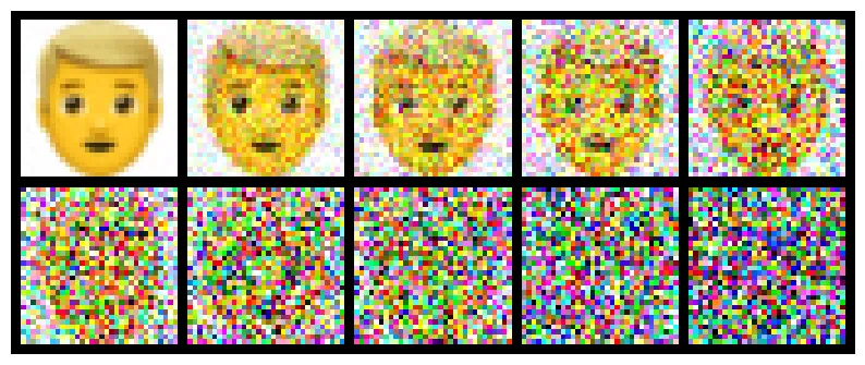
타임스텝이 따라 이미지에 노이즈가 더해지는것을 확인할 수 있다.

predict_start_from_noise

pred_noise objective에서는 U-Net이 $x_0$가 아니라 noise $\epsilon$을 예측한다. 하지만 Reverse Diffusion에서 q_posterior(x_start, x_t, t)를 계산하려면 $x_0$의 추정값이 필요하므로, 모델이 예측한 noise와 현재 $x_t$를 이용해 $x_0$를 복원해야 한다.

Forward Diffusion 식은 다음과 같다.

$$x_t = \sqrt{\bar{\alpha}_t}x_0 + \sqrt{1-\bar{\alpha}_t}\epsilon$$

이를 $x_0$에 대해 정리하면 다음과 같다.

$$x_0 = \frac{ x_t-\sqrt{1-\bar{\alpha}_t}\epsilon }{ \sqrt{\bar{\alpha}_t} }$$

def predict_start_from_noise(self, x_t, t, noise):
    sqrt_alpha_bar_t = extract(self.sqrt_alphas_cumprod, t, x_t.shape)

    sqrt_one_minus_alpha_bar_t = extract(self.sqrt_one_minus_alphas_cumprod, t, x_t.shape)

    x_start = (x_t - sqrt_one_minus_alpha_bar_t * noise) / sqrt_alpha_bar_t

    return x_start

predict_noise_from_start

pred_x_start objective에서는 U-Net이 noise가 아니라 $x_0$를 직접 예측한다. 따라서 $x_t$와 예측된 $x_0$로부터 noise $\epsilon$이 필요한 경우 다시 계산할 수 있어야 한다.

모델이 pred_noise와 pred_x_start 중 어느 objective를 사용하더라도 $x_0$와 noise 표현 사이를 서로 변환할 수 있도록 하기 위한 함수이다. 현재 p_sample 구현에서는 pred_x_start일 때 $x_0$를 바로 q_posterior에 사용할 수 있으므로 필수적으로 호출되는것은 아니다.

Forward Diffusion 식을 $\epsilon$에 대해 정리하면 다음과 같다.

$$\epsilon = \frac{ x_t-\sqrt{\bar{\alpha}_t}x_0 }{ \sqrt{1-\bar{\alpha}_t} }$$

def predict_noise_from_start(self, x_t, t, x_start):
    sqrt_alpha_bar_t = extract(self.sqrt_alphas_cumprod, t, x_t.shape)

    sqrt_one_minus_alpha_bar_t = extract(self.sqrt_one_minus_alphas_cumprod, t, x_t.shape)

    pred_noise = (x_t - sqrt_alpha_bar_t * x_start) / sqrt_one_minus_alpha_bar_t

    return pred_noise

U-Net 모델

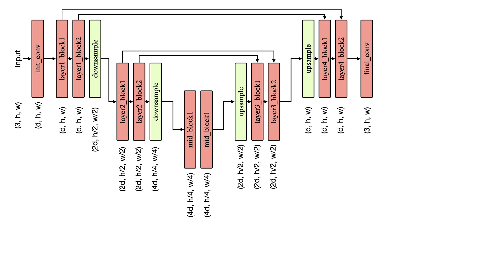
DDPM에서 U-Net은 현재 노이즈가 섞인 이미지 $x_t$를 입력받아 noise를 예측하는 denoising model로 사용된다.

$$\hat{\epsilon} = \epsilon_\theta(x_t,t,c)$$

Diffusion에서는 입력과 출력이 모두 이미지 형태이므로 공간 정보를 유지하면서 각 위치의 noise를 예측해야 한다. U-Net은 Downsampling을 통해 해상도를 줄이면서 점점 더 high-level feature를 추출하고, Upsampling을 통해 다시 원래 해상도로 복원한다.

Downsampling 과정에서는 해상도가 감소하는 대신 채널 수를 증가시켜 더 많은 feature를 표현한다.

$$(B,C,H,W) \rightarrow (B,C',H/2,W/2)$$

반대로 Upsampling에서는 해상도를 다시 증가시키고 채널 수를 감소시킨다.

$$(B,C,H,W) \rightarrow (B,C',2H,2W)$$

이 과정에서 Downsampling을 거치며 세밀한 공간 정보가 손실될 수 있기 때문에 각 ResNet block의 feature map을 Skip Connection으로 저장한다. Upsampling에서는 같은 해상도의 특징과 concatenate하여 Downsampling에서 보존한 정보를 다시 사용한다.

$$\operatorname{Concat}(x,\text{skip}) : (B,C,H,W)+(B,C,H,W) \rightarrow (B,2C,H,W)$$

이후 ResNet block이 concatenate된 feature를 처리하면서 다시 원래 채널 수로 줄인다.

$$(B,2C,H,W) \rightarrow (B,C,H,W)$$

따라서 U-Net은 전체적인 구조를 파악하는 high-level feature와 경계, 위치와 같은 세밀한 공간 정보를 함께 이용할 수 있어 image denoising에 적합하다.

또한 이 구현에서는 timestep embedding과 text embedding을 context로 만들어 각 ResNet block에 전달한다. 따라서 U-Net은 현재 이미지 $x_t$뿐만 아니라 현재 noise level $t$와 condition $c$를 함께 고려해 예측을 수행한다.

Downsampling / Upsampling Block 구성

dims = [dim] + [dim * m for m in dim_mults]
in_out = list(zip(dims[:-1], dims[1:]))
in_out_ups = [(b, a) for a, b in reversed(in_out)]

context_dim = dim * 4

self.downs = nn.ModuleList([])
self.ups = nn.ModuleList([])

for ind, (dim_in, dim_out) in enumerate(in_out):
    down_block = nn.ModuleList([
        ResnetBlock(dim_in, dim_in, context_dim=context_dim),
        ResnetBlock(dim_in, dim_in, context_dim=context_dim),
        Downsample(dim_in, dim_out),
    ])

    self.downs.append(down_block)

mid_dim = dims[-1]
self.mid_block1 = ResnetBlock(mid_dim, mid_dim, context_dim=context_dim)
self.mid_block2 = ResnetBlock(mid_dim, mid_dim, context_dim=context_dim)

for ind, (dim_in, dim_out) in enumerate(in_out_ups):
    up_block = nn.ModuleList([
        Upsample(dim_in, dim_out),
        ResnetBlock(dim_out * 2, dim_out, context_dim=context_dim),
        ResnetBlock(dim_out * 2, dim_out, context_dim=context_dim),
    ])

    self.ups.append(up_block)

Downsampling block은 두 개의 ResNet block에서 feature를 추출한 뒤 Downsample을 통해 해상도를 절반으로 줄이고 채널 수를 증가시킨다.

Upsampling block에서는 먼저 해상도를 두 배로 늘린 뒤 Skip Connection을 concatenate한다. 이 때문에 각 ResNet block의 입력 채널 수는 2 * dim_out이 되고, ResNet block을 통과하면서 다시 dim_out 채널로 정리된다.

forward

def forward(self, x, time, model_kwargs={}):
    if "cfg_scale" in model_kwargs:
        return self.cfg_forward(x, time, model_kwargs)

    context = self.time_mlp(time)

    cond_emb = model_kwargs["text_emb"]
    if cond_emb is None:
        cond_emb = torch.zeros(x.shape[0], self.condition_dim, device=x.device)

    if self.training:
        mask = (torch.rand(cond_emb.shape[0]) > self.uncond_prob).float()
        mask = mask[:, None].to(cond_emb.device)
        cond_emb = cond_emb * mask

    context = context + self.condition_mlp(cond_emb)

    x = self.init_conv(x)

    h = []

    for block1, block2, downsample in self.downs:
        # x: (B, dim_in, H, W)

        x = block1(x, context) # x: (B, dim_in, H, W)

        h.append(x)
        x = block2(x, context) # x: (B, dim_in, H, W)
        h.append(x)

        x = downsample(x) # x: (B, dim_out, H/2, W/2)

    x = self.mid_block1(x, context) # x: (B, mid_dim, H_min, W_min)
    x = self.mid_block2(x, context) # x: (B, mid_dim, H_min, W_min)

    for upsample, block1, block2 in self.ups:
        # x: (B, dim_in, H, W)

        x = upsample(x) # x: (B, dim_out, 2H, 2W)

        x = torch.cat((x, h.pop()), dim=1)
        # x: (B, dim_out, 2H, 2W)
        # skip: (B, dim_out, 2H, 2W)
        # concat: (B, 2*dim_out, 2H, 2W)

        x = block1(x, context) # x: (B, dim_out, 2H, 2W)

        x = torch.cat((x, h.pop()), dim=1)
        # x: (B, dim_out, 2H, 2W)
        # skip: (B, dim_out, 2H, 2W)
        # concat: (B, 2*dim_out, 2H, 2W)

        x = block2(x, context) # x: (B, dim_out, 2H, 2W)

    x = self.final_conv(x)

    return x

Downsampling 단계에서는 각 ResNet block의 출력을 h에 저장한다. 한 Downsampling block마다 두 개의 ResNet block이 있으므로 Skip Connection에 사용할 feature도 두 개씩 저장된다.

Upsampling에서는 가장 깊은 feature부터 사용해야 하므로 h.pop()으로 저장된 feature를 역순으로 꺼낸다.

전체 흐름은 다음과 같다.

$$x_t \rightarrow \text{Downsampling} \rightarrow \text{Middle} \rightarrow \text{Upsampling + Skip Connection} \rightarrow \hat{\epsilon}$$

p_losses

p_losses는 DDPM을 학습할 때 loss를 계산하는 함수이다. Clean image $x_0$에서 임의의 timestep $t$를 선택하고, q_sample을 이용해 해당 timestep의 noisy image $x_t$를 만든다. 이후 U-Net이 $x_t$를 입력받아 target을 예측하도록 학습한다.

이번 구현에서는 objective에 따라 target이 달라진다.

• pred_noise: Forward Diffusion에 사용한 noise $\epsilon$을 예측한다.
• pred_x_start: 원본 이미지 $x_0$를 직접 예측한다.

pred_noise일 때 학습 흐름은 다음과 같다.

$$x_0 \xrightarrow{q(x_t \mid x_0)} x_t \xrightarrow{\epsilon_\theta(x_t,t,c)} \hat{\epsilon} \xrightarrow{\mathrm{MSE}} \mathcal{L}$$

먼저 batch의 각 이미지마다 임의의 timestep $t$를 선택한다.

$$t \sim \mathrm{Uniform}(0,T-1)$$

그다음 Gaussian noise를 생성한다.

$$\epsilon \sim \mathcal{N}(0,I)$$

q_sample을 이용해 $x_0$에서 해당 timestep의 $x_t$를 바로 생성한다.

$$x_t = \sqrt{\bar{\alpha}_t}x_0 + \sqrt{1-\bar{\alpha}_t}\epsilon$$

이 $x_t$와 timestep $t$를 U-Net에 입력한다.

$$\hat{\epsilon} = \epsilon_\theta(x_t,t,c)$$

pred_noise objective에서는 Forward Diffusion에 실제로 사용한 noise $\epsilon$과 U-Net이 예측한 noise $\hat{\epsilon}$ 사이의 MSE를 최소화한다.

$$\mathcal{L} = \mathbb{E}_{t,x_0,\epsilon} \left[ w_t \left\| \epsilon - \epsilon_\theta \left( \sqrt{\bar{\alpha}_t}x_0 + \sqrt{1-\bar{\alpha}_t}\epsilon, t \right) \right\|^2 \right]$$

여기서 $w_t$는 timestep별 loss_weight이다. pred_noise에서는 기본적으로 모든 timestep의 weight가 1이고, pred_x_start에서는 SNR(Signal-to-Noise Ratio)에 따라 weight가 달라진다.

reduction="none"을 사용하는 이유는 MSE를 바로 하나의 scalar로 줄이지 않고 각 원소의 loss를 유지한 상태에서 timestep별 loss_weight를 먼저 적용하기 위해서이다.

$$(B,C,H,W) \times (B,1,1,1) \rightarrow (B,C,H,W)$$

각 배치 샘플에 해당하는 하나의 weight가 모든 채널과 공간 위치에 브로드캐스팅된다. 마지막에 .mean()을 적용해 전체 loss를 하나의 scalar로 만든다.

구현

def p_losses(self, x_start, model_kwargs={}):
    b, nts = x_start.shape[0], self.num_timesteps
    t = torch.randint(0, nts, (b,), device=x_start.device).long()  # (b,)
    x_start = self.normalize(x_start)  # (b, *)
    noise = torch.randn_like(x_start)  # (b, *)
    target = noise if self.objective == "pred_noise" else x_start  # (b, *)
    loss_weight = extract(self.loss_weight, t, target.shape)  # (b, *)
    loss = None

    x_t = self.q_sample(x_start, t, noise)
    model_pred = self.model(x_t, t, model_kwargs=model_kwargs)
    loss = nn.functional.mse_loss(model_pred, target, reduction="none")
    loss = (loss * loss_weight).mean()

    return loss

전체 흐름은 다음과 같다.

$$x_0 \rightarrow \text{Random timestep }t \rightarrow \text{Gaussian noise }\epsilon \rightarrow q_\text{sample} \rightarrow x_t \rightarrow \text{U-Net} \rightarrow \text{Prediction} \rightarrow \text{Weighted MSE}$$

p_losses는 Forward Diffusion으로 학습에 사용할 noisy image를 만들고, U-Net의 prediction이 target noise 또는 원본 이미지에 가까워지도록 loss를 계산하는 역할을 한다.

p_sample

p_sample은 DDPM의 inference 과정에서 현재 noisy image $x_t$로부터 한 단계 덜 noisy한 $x_{t-1}$을 샘플링하는 함수이다.

학습 과정의 q_sample이 $x_0$에서 $x_t$를 만드는 Forward Diffusion이라면 p_sample은 반대로 $x_t$에서 $x_{t-1}$을 생성하는 Reverse Diffusion의 한 step을 담당한다.

전체 샘플링 과정에서는 Gaussian noise $x_T$에서 시작해 p_sample을 반복적으로 호출한다.

$$x_T \rightarrow x_{T-1} \rightarrow x_{T-2} \rightarrow \cdots \rightarrow x_0$$

먼저 현재 $x_t$와 timestep $t$를 U-Net에 입력해 model prediction을 얻는다.

pred_noise objective에서는 U-Net이 noise $\epsilon$을 예측한다.

$$\hat{\epsilon} = \epsilon_\theta(x_t,t,c)$$

하지만 posterior distribution을 계산하려면 $x_0$의 추정값이 필요하기 때문에, predict_start_from_noise를 이용해 predicted noise로부터 $x_0$를 복원한다.

$$\hat{x}_0 = \frac{ x_t - \sqrt{1-\bar{\alpha}_t}\hat{\epsilon} }{ \sqrt{\bar{\alpha}_t} }$$

반대로 pred_x_start objective에서는 U-Net이 $x_0$를 직접 예측하므로 model prediction을 그대로 사용한다.

예측한 $x_0$는 정규화된 이미지 범위를 벗어나지 않도록 $[-1,1]$로 clamp(정해진 범위 안으로 자름)한다.

$$\hat{x}_0 \leftarrow \operatorname{clip}(\hat{x}_0,-1,1)$$

이후 q_posterior를 이용해 $x_t$와 추정된 $x_0$가 주어졌을 때 $x_{t-1}$의 posterior distribution을 계산한다.

$$q(x_{t-1}\mid x_t,x_0) = \mathcal{N} \left( x_{t-1}; \tilde{\mu}_t(x_t,x_0), \tilde{\beta}_t I \right)$$

코드에서는 이 분포의 평균과 표준편차를 posterior_mean, posterior_std로 얻는다.

마지막으로 Gaussian noise를 이용해 $x_{t-1}$을 샘플링한다.

$$x_{t-1} = \text{posterior\_mean} + \text{posterior\_std}\cdot z$$

여기서 $z$는 다음과 같이 샘플링한다.

$$z \sim \mathcal{N}(0,I)$$

마지막 timestep $t=0$에서는 더 이상 노이즈를 추가할 필요가 없으므로 $z=0$으로 두고 posterior mean을 그대로 사용한다.

구현

@torch.no_grad()
def p_sample(self, x_t, t: int, model_kwargs={}):
    t = torch.full(
        (x_t.shape[0],),
        t,
        device=x_t.device,
        dtype=torch.long
    )  # (b,)

    x_tm1 = None

    model_pred = self.model(x_t, t, model_kwargs=model_kwargs)

    if self.objective == "pred_noise":
        x_start = self.predict_start_from_noise(x_t, t, model_pred)
    else:
        x_start = model_pred

    x_start = x_start.clamp(-1, 1)

    posterior_mean, posterior_std = self.q_posterior(
        x_start, x_t, t
    )

    noise = torch.randn_like(x_t) if t[0] > 0 else 0
    x_tm1 = posterior_mean + posterior_std * noise

    return x_tm1

전체 흐름은 다음과 같다.

$$x_t \rightarrow \text{U-Net Prediction} \rightarrow \hat{x}_0 \rightarrow q(x_{t-1}\mid x_t,\hat{x}_0) \rightarrow x_{t-1}$$

p_sample은 U-Net의 prediction을 이용해 $x_0$를 추정하고, 이를 바탕으로 posterior distribution을 계산한 뒤 $x_{t-1}$을 샘플링하는 Reverse Diffusion의 한 단계다.

Training

훈련의 핵심은 batch를 가져와 p_losses로 DDPM loss를 계산하고, 역전파를 수행해 U-Net의 파라미터를 업데이트하는 과정이다.

전체 흐름은 다음과 같다.

$$\text{Batch} \rightarrow p\_\text{losses} \rightarrow \text{Loss} \rightarrow \text{Backward} \rightarrow \text{Optimizer Step}$$

먼저 이미지와 text embedding을 device로 이동한다.

data, model_kwargs = next(self.dl)
data = data.to(device)
model_kwargs["text_emb"] = model_kwargs["text_emb"].to(device)

이후 p_losses에서 noisy image를 생성하고 U-Net prediction과 target 사이의 loss를 계산한다.

self.opt.zero_grad()

loss = self.diffusion_model.p_losses(
    data,
    model_kwargs=model_kwargs
)

loss.backward()

torch.nn.utils.clip_grad_norm_(
    self.diffusion_model.parameters(),
    1.0
)

self.opt.step()

zero_grad()로 이전 gradient를 초기화하고, backward()로 gradient를 계산한 뒤 optimizer.step()으로 파라미터를 업데이트한다.

clip_grad_norm_은 gradient norm이 너무 커지는 것을 제한해 학습을 안정화한다.

일정 step마다 체크포인트를 저장하고 현재 모델로 이미지를 샘플링한다.

if self.step % self.save_every == 0:
    self.save(self.step)

if self.step % self.sample_every == 0:
    self.diffusion_model.eval()

    with torch.no_grad():
        model_kwargs = self.ds.random_model_kwargs(self.num_samples)
        model_kwargs["text_emb"] = model_kwargs["text_emb"].to(device)

        all_images = self.diffusion_model.sample(
            batch_size=self.num_samples,
            model_kwargs=model_kwargs
        )

실제 학습의 핵심은 다음 네 단계이다.

self.opt.zero_grad()
loss = self.diffusion_model.p_losses(data, model_kwargs=model_kwargs)
loss.backward()
self.opt.step()

p_losses 내부에서 Forward Diffusion과 U-Net prediction이 수행되므로, Trainer는 계산된 loss를 이용해 파라미터를 반복적으로 업데이트하는 역할을 한다.

sample

sample은 p_sample을 모든 timestep에 대해 반복하여 최종 이미지를 생성하는 함수이다. 처음에는 이미지와 같은 shape의 Gaussian noise $x_T$를 생성한다.

$$x_T \sim \mathcal{N}(0,I)$$

이후 timestep을 역순으로 순회하며 p_sample을 호출한다.

@torch.no_grad()
def sample(self, batch_size=16, return_all_timesteps=False, model_kwargs={}):
    shape = (
        batch_size,
        self.channels,
        self.image_size,
        self.image_size
    )

    img = torch.randn(shape, device=self.betas.device)
    imgs = [img]

    for t in tqdm(
        reversed(range(0, self.num_timesteps)),
        desc="sampling loop time step",
        total=self.num_timesteps,
    ):
        img = self.p_sample(img, t, model_kwargs=model_kwargs)
        imgs.append(img)

    res = img if not return_all_timesteps else torch.stack(imgs, dim=1)
    res = self.unnormalize(res)

    return res

따라서 p_sample이 Reverse Diffusion의 한 step이라면, sample은 이 step을 반복하여 Gaussian noise에서 최종 이미지를 생성하는 전체 샘플링 과정이다.

$$x_T \xrightarrow{p_\theta} x_{T-1} \xrightarrow{p_\theta} \cdots \xrightarrow{p_\theta} x_1 \xrightarrow{p_\theta} x_0$$

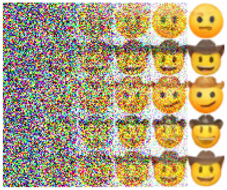
Gaussian noise에서 시작해 Reverse Diffusion을 반복하면서 점차 이모지 이미지가 생성되는 샘플링 과정을 보여준다.

cfg_forward

def cfg_forward(self, x, time, model_kwargs={}):
    cfg_scale = model_kwargs.pop("cfg_scale")
    print("Classifier-free guidance scale:", cfg_scale)
    model_kwargs = copy.deepcopy(model_kwargs)

    cond_pred = self.forward(x, time, model_kwargs=model_kwargs)

    uncond_kwargs = copy.deepcopy(model_kwargs)
    uncond_kwargs["text_emb"] = None
    uncond_pred = self.forward(x, time, model_kwargs=uncond_kwargs)

    x = (cfg_scale + 1) * cond_pred - cfg_scale * uncond_pred

    return x

Classifier-Free Guidance에서는 동일한 U-Net을 두 번 호출해 Conditional Prediction과 Unconditional Prediction을 얻는다.

$$\epsilon_{\mathrm{cond}} = \epsilon_\theta(x_t,t,c)$$ $$\epsilon_{\mathrm{uncond}} = \epsilon_\theta(x_t,t,\phi)$$

두 prediction의 차이를 이용해 condition의 영향을 강화한다.

$$\epsilon_\theta(x_t,t,c) \leftarrow (w+1)\epsilon_\theta(x_t,t,c) - w\epsilon_\theta(x_t,t,\phi)$$

동일한 식은 다음처럼 볼 수 있다.

$$\epsilon_{\mathrm{CFG}} = \epsilon_{\mathrm{cond}} + w \left( \epsilon_{\mathrm{cond}} - \epsilon_{\mathrm{uncond}} \right)$$

Conditional Prediction을 기본으로 사용하면서 Conditional Prediction과 Unconditional Prediction의 차이를 guidance scale $w$만큼 추가해 condition 방향을 강화한다.

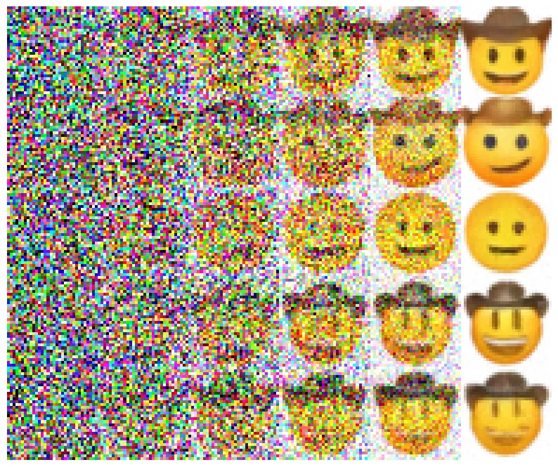Classifier-Free Guidance scale을 1로 설정한 샘플링 결과이다. 초기 Gaussian noise에서 시작해 Reverse Diffusion을 반복하면서 점차 이모지의 형태와 표정이 드러나는 것을 확인할 수 있다.

$$\epsilon_\theta(x_t,t,c) \leftarrow 2\epsilon_\theta(x_t,t,c) - \epsilon_\theta(x_t,t,\phi)$$

$w=1$이므로 Conditional Prediction과 Unconditional Prediction의 차이를 한 번 추가해 condition의 영향을 강화한다.

추가 개념들

SNR

SNR(Signal-to-Noise Ratio)은 현재 timestep에서 원본 이미지 성분과 noise 성분의 비율을 나타낸다.

$$\mathrm{SNR}(t) = \frac{\bar{\alpha}_t} {1-\bar{\alpha}_t}$$

초기 timestep에서는 원본 이미지 성분이 많이 남아 있으므로 SNR이 크고, timestep이 커질수록 noise 비중이 증가하면서 SNR이 작아진다.

q_posterior

q_posterior는 현재 noisy image $x_t$와 추정한 원본 이미지 $\hat{x}_0$를 이용해 한 단계 이전 상태인 $x_{t-1}$의 posterior distribution을 계산한다.

$$q(x_{t-1}\mid x_t,x_0) = \mathcal{N} \left( x_{t-1}; \tilde{\mu}_t(x_t,x_0), \tilde{\beta}_t I \right)$$

p_sample에서는 이 분포의 평균과 표준편차를 구한 뒤 Gaussian noise를 이용해 $x_{t-1}$을 샘플링한다.