
Overview
Transformer 의 Multi-Headed Attention 을 구현하고, Positional Encoding 의 원리와 구현, Transformer Block 을 만들고 COCO Dataset 으로 이미지 캡셔닝과 ViT를 구현한다.
Multi-Headed Attention
Multi-Headed Attention은 embedding을 여러 head로 나누어 각 head가 서로 다른 표현 공간에서 token 사이의 관계를 포착하도록 한다.
각 head의 attention은 다음과 같이 계산된다.
각 head의 출력을 다시 연결한 뒤 output projection을 적용한다.
Cross-Attention
Cross-Attention은 서로 다른 입력에서 Query와 Key/Value를 구성하고, 각각을 attention 계산이 가능한 표현 공간으로 projection하여 두 입력 사이의 관계를 포착한다.
Positional Encoding
Self-Attention 자체는 token의 순서나 위치를 알 수 없으므로 embedding에 positional encoding을 더해 위치 정보를 제공한다.
ViT에서는 이 위치 정보가 각 image patch의 공간적 위치를 구분하는 역할을 한다.
Image Captioning
이미지 feature를 decoder가 참고할 memory로 변환하고, caption token 은 embedding과 positional encoding을 거쳐 target이 된다.
이후 디코더가 target, memory을 이용하여 attention 연산을 적용하고, n번째(batch) caption의 t번째 위치에서 vocab V개에 대한 점수를 생성한다.
Encoder 와 Decoder
인코더는 입력 전체를 보고 각 token의 문맥이 반영된 representation을 만든다. 입력 전체가 이미 주어져 있으므로 일반적으로 모든 token이 서로 self-attention할 수 있으며, 분류나 feature extraction 등에 주로 사용된다.
이번 과제에서의 대략적인 인코더 구조는 다음과 같다.
%% title: Transformer Encoder 구조
%% caption: Self-Attention과 FFN 뒤에 dropout, residual connection, layer normalization을 적용한다.
flowchart LR
    input["Input"] --> attention["Self-Attention"]
    attention --> residual1["Dropout<br/>+ Residual"]
    residual1 --> norm1["LayerNorm"]
    norm1 --> ffn["FFN"]
    ffn --> dropout["Dropout"]
    dropout --> residual2["Residual"]
    residual2 --> norm2["LayerNorm"]
디코더는 encoded representation을 목표 출력으로 변환하는 역할을 하며, Encoder-Decoder Transformer에서 디코더는 이전 target token과 Encoder의 representation을 이용하여 target sequence를 autoregressive하게 생성한다.
autoregressive: 이전 출력들을 이용해서 다음 출력을 순차적으로 예측하는 방식
이번 과제에서의 대략적인 디코더 구조는 다음과 같다.
%% title: Transformer Decoder 구조
%% caption: Masked Self-Attention으로 이전 target을 처리하고 Cross-Attention으로 encoder의 memory를 참고한 뒤 FFN을 통과한다.
flowchart LR
    input["Input"] --> masked["Masked<br/>Self-Attention"]
    masked --> residual1["Dropout<br/>+ Residual"]
    residual1 --> norm1["LayerNorm"]
    norm1 --> cross["Cross-Attention"]
    cross --> residual2["Dropout<br/>+ Residual"]
    residual2 --> norm2["LayerNorm"]
    norm2 --> ffn["FFN"]
    ffn --> residual3["Dropout<br/>+ Residual"]
    residual3 --> norm3["LayerNorm"]
여기서 Cross-Attention은 Decoder의 현재 representation(target)을 Query로 사용하고, Encoder의 출력인 memory를 Key와 Value로 사용한다.
이번 과제의 Cross-Attention은 현재 caption representation을 Query로 하고 하나의 global image representation을 Key와 Value로 사용하여, 이미지 정보를 각 target representation에 결합한다.
(직관적으로, caption 문맥을 Query로 사용해서 이미지 한 장 안의 여러 visual token 중 현재 문맥과 관련 있는 정보에 더 큰 attention을 주고, 그 정보를 caption representation에 반영한다.)
일반적인 image captioning Transformer에서 image memory가 여러 visual token으로 구성되는 경우에는 Query에 따라 관련 visual token들을 서로 다른 가중치로 가중합하여 현재 문맥에 필요한 visual context를 구성할 수 있다.
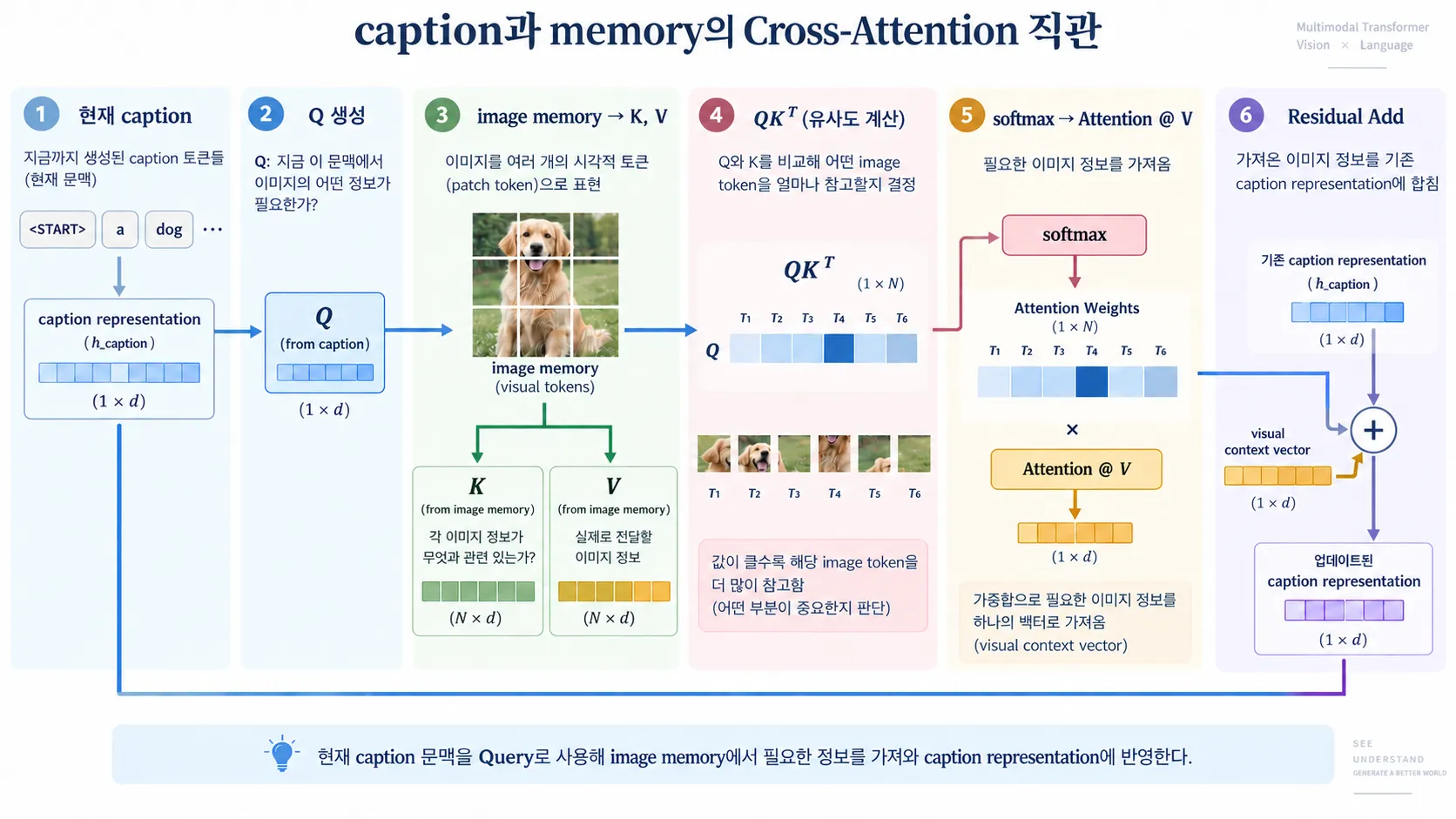
caption과 memory의 Cross-Attention 직관
현재 caption
-> Q: "지금 이 문맥에서 이미지의 어떤 정보가 필요한가?"

image memory
-> K: "각 이미지 정보가 무엇과 관련 있는가?"
-> V: "실제로 전달할 이미지 정보"

Q와 K 비교
-> 어떤 image token을 얼마나 참고할지 결정

Attention @ V
-> 필요한 이미지 정보를 가져옴

Residual Add
-> 가져온 이미지 정보를 기존 caption representation에 합침| Transformer Encoder | Transformer Decoder | |
|---|---|---|
| 주목적 | 입력 전체를 이해하고 representation 생성 | 순차적으로 다음 token 생성 |
| Self-Attention | 모든 token이 서로 볼 수 있음 | 보통 미래 token을 못 보게 causal mask 사용 |
| Cross-Attention | 없음 | Encoder-Decoder 구조에서는 존재 |
| 입력 | 완성된 입력 sequence | 지금까지 생성된 token sequence |
| 대표 용도 | 분류, feature extraction, ViT | 언어 생성, caption 생성 |
구현
Multi-Head Attention
멀티헤드 어텐션은 세 가지 분기로 처리했다. 단순히 Q,K,V 를 각각 proj 한 후 축을 바꾸고 어텐션 연산을 수행해도 되지만, self-attention 인 경우에 fused attention 을 구현했다.
각각 위 연산을 계산하는 대신 weight를 아래처럼 합친다.
이후 한 번에 계산한 뒤 결과를 , , 로 분할한다.
class MultiHeadAttention(nn.Module):
    """
    A model layer which implements a simplified version of masked attention, as
    introduced by "Attention Is All You Need" (https://arxiv.org/abs/1706.03762).

    Usage:
      attn = MultiHeadAttention(embed_dim, num_heads=2)

      # self-attention
      data = torch.randn(batch_size, sequence_length, embed_dim)
      self_attn_output = attn(query=data, key=data, value=data)

      # attention using two inputs
      other_data = torch.randn(batch_size, sequence_length, embed_dim)
      attn_output = attn(query=data, key=other_data, value=other_data)
    """

    def __init__(self, embed_dim, num_heads, dropout=0.1):
        """
        Construct a new MultiHeadAttention layer.

        Inputs:
         - embed_dim: Dimension of the token embedding
         - num_heads: Number of attention heads
         - dropout: Dropout probability
        """
        super().__init__()
        assert embed_dim % num_heads == 0

        self.key = nn.Linear(embed_dim, embed_dim)
        self.query = nn.Linear(embed_dim, embed_dim)
        self.value = nn.Linear(embed_dim, embed_dim)
        self.proj = nn.Linear(embed_dim, embed_dim)

        self.attn_drop = nn.Dropout(dropout)

        self.n_head = num_heads
        self.emd_dim = embed_dim
        self.head_dim = self.emd_dim // self.n_head

    def forward(self, query, key, value, attn_mask=None):
        """
        Calculate the masked attention output for the provided data, computing
        all attention heads in parallel.

        In the shape definitions below, N is the batch size, S is the source
        sequence length, T is the target sequence length, and E is the embedding
        dimension.

        Inputs:
        - query: Input data to be used as the query, of shape (N, S, E)
        - key: Input data to be used as the key, of shape (N, T, E)
        - value: Input data to be used as the value, of shape (N, T, E)
        - attn_mask: Array of shape (S, T) where mask[i,j] == 0 indicates token
          i in the source should not influence token j in the target.

        Returns:
        - output: Tensor of shape (N, S, E) giving the weighted combination of
          data in value according to the attention weights calculated using key
          and query.
        """
        N, S, E = query.shape
        N, T, E = value.shape
        # Create a placeholder, to be overwritten by your code below.
        output = torch.empty((N, S, E))

        H = self.n_head
        D_h = self.head_dim

        # Q, K, V 프로젝션만 분기 처리
        # self-attention
        if query is key and key is value:
          # S == T
          # (3E, E)
          weight = torch.cat([
            self.query.weight,
            self.key.weight,
            self.value.weight,
          ], dim=0)

          # (3E,)
          bias = torch.cat([
            self.query.bias,
            self.key.bias,
            self.value.bias
          ], dim=0)

          # query == key == value
          # xW^T + b:
          # (N, T, E) @ (E, 3E) -> (N, T, 3E)
          qkv = F.linear(query, weight, bias)

          # (N, T, 3E) -> (N, T, 3, H, E/H) -> Q, K, V each (N, T, H, E/H)
          Q, K, V = qkv.reshape(N, T, 3, H, D_h).unbind(dim=2)

          # permute
          # (N, T, H, E/H) -> (N, H, T, E/H)
          Q = Q.permute(0, 2, 1, 3)
          K = K.permute(0, 2, 1, 3)
          V = V.permute(0, 2, 1, 3)

        # cross-attention
        elif key is value:
          # Q, KV
          # (N, S, E) @ (E, E) -> (N, S, E)
          Q = self.query(query)

          # (2E, E)
          kv_weight = torch.cat([self.key.weight, self.value.weight], dim=0)
          # (2E,)
          kv_bias = torch.cat([self.key.bias, self.value.bias], dim=0)

          # (N, T, E) @ (E, 2E) -> (N, T, 2E)
          KV = F.linear(key, kv_weight, kv_bias)

          # (N, S, E) -> (N, S, H, D_h)
          Q = Q.reshape(N, S, H, D_h)
          # (N, T, 2E) -> (N, T, 2, H, D_h) -> (N, T, H, D_h)
          K, V = KV.reshape(N, T, 2, H, D_h).unbind(dim=2)

          # permute
          # (N, S, H, E/H) -> (N, H, S, E/H)
          Q = Q.permute(0, 2, 1, 3)

          # (N, T, H, E/H) -> (N, H, T, E/H)
          K = K.permute(0, 2, 1, 3)
          V = V.permute(0, 2, 1, 3)

        else:
          Q = self.query(query).reshape(N, S, H, D_h)
          K = self.key(key).reshape(N, T, H, D_h)
          V = self.value(value).reshape(N, T, H, D_h)

          # permute
          # (N, S, H, E/H) -> (N, H, S, E/H)
          Q = Q.permute(0, 2, 1, 3)

          # (N, T, H, E/H) -> (N, H, T, E/H)
          K = K.permute(0, 2, 1, 3)
          V = V.permute(0, 2, 1, 3)

        # ====== Attention ======
        # (N, H, S, E/H) @ (N, H, E/H, T) -> (N, H, S, T)
        scores = (Q @ K.transpose(-2, -1)) / math.sqrt(D_h)

        # attn_mask: (S, T)
        if attn_mask is not None:
          scores = scores.masked_fill(attn_mask == 0, float("-inf"))

        attn = F.softmax(scores, dim=-1)
        attn = self.attn_drop(attn)

        # (N, H, S, T) @ (N, H, T, E/H) -> (N, H, S, E/H)
        context = attn @ V

        # (N, H, S, E/H) -> (N, S, H, E/H) -> (N, S, H * E/H) = (N, S, E)
        attn_output = context.permute(0, 2, 1, 3).reshape(N, S, E)

        # (N, S, E) @ (E, E) -> (N, S, E)
        output = self.proj(attn_output)

        return output
Positional Encording
Positional Encording 의 경우 먼저 짝수 차원 에 대해 로그의 기본 성질인 성질을 이용하여 를 형태의 주파수 벡터를 만든다.
이후 token 의 위치 를 나타내는 position vector와 주파수 벡터를 브로드캐스팅 하여 를 모든 위치와 차원에 대하여 한번씩 계산한다.
이 결과에 대해 짝수 channel에는 , 바로 다음 홀수 channel에는 같은 주파수의 를 적용한다.
따라서 인접한 짝수·홀수 channel은 같은 주파수를 공유하며, 최종적으로 형태의 positional encoding matrix가 만들어진다.
이 행렬을 token embedding 에 더해 위치 정보를 주입한다.
코드에서는 positional encoding을 매 forward마다 다시 계산하지 않고, 최대 sequence 길이까지 미리 만들어 둔다. 이라고 하면 저장하는 배열의 shape은 다음과 같다.
- 첫 번째 축 은 batch broadcasting을 위한 축이다.
- 두 번째 축 은 token의 position을 나타낸다.
- 세 번째 축 는 embedding channel을 나타낸다.
따라서 PE[0, i, j]는 번째 token position의 번째 embedding channel에 더할 값이다.
Position vector
각 token의 위치 를 만들기 위해 다음 코드를 사용한다.
position = torch.arange(max_len).unsqueeze(1)torch.arange(max_len)은 다음 vector를 만든다.
이때 shape은 이다. unsqueeze(1)로 두 번째 축을 추가하면 다음과 같은 column vector가 된다.
각 행은 token position 하나에 대응한다.
Frequency vector
다음 코드는 짝수 embedding channel 에 사용할 index를 만든다.
torch.arange(0, embed_dim, 2)가 짝수라면 결과는 이고 shape은 이다. Sinusoidal positional encoding에 필요한 는 를 이용해 다음과 같이 계산한다.
div_term = torch.exp(
    torch.arange(0, embed_dim, 2)
    * (-math.log(10000.0) / embed_dim)
)
따라서 div_term의 shape은 이며, 내부에는 다음 주파수 값들이 들어 있다.
번째 값을 라고 두면 div_term은 와 같이 서로 다른 주파수를 담은 vector이다.
Position과 frequency의 broadcasting
position 과 div_term을 곱하면 다음 shape 변화가 생긴다.
position * div_termBroadcasting은 shape을 오른쪽 축부터 비교하며, 각 축의 크기가 같거나 둘 중 하나가 이면 적용될 수 있다. 여기서 는 로 오른쪽 정렬되므로 과 연산하면 로 확장된다.
PyTorch broadcasting에 의해 모든 position과 모든 주파수의 조합이 한 번에 계산된다.
결과 행렬의 번째 원소는 이다.
Sine과 cosine을 channel에 대입하기
PE[:, :, 0::2]는 마지막 축에서 인 짝수 channel만 선택한다. 이 view의 shape은 이다.
pe[:, :, 0::2] = torch.sin(position * div_term)오른쪽 값의 shape 은 첫 번째 축으로 broadcasting되어 짝수 channel에 들어간다.
PE[:, :, 0::2]에서 앞의 두 :는 batch 축과 position 축의 모든 index를 선택하고, 0::2는 마지막 축의 짝수 channel만 선택한다. 따라서 의 shape이 라면 PE[:, :, 0::2]의 shape은 이다.
우변인 position * div_term의 shape 은 앞에 크기 인 축이 추가된 것처럼 broadcasting된다. 이때 각 원소는 다음과 같이 대응하며, PyTorch가 이 대입을 하나의 tensor 연산으로 처리한다.
PE[:, :, 1::2]는 인 홀수 channel만 선택하며, 짝수 channel과 동일한 position * div_term을 사용한다.
pe[:, :, 1::2] = torch.cos(position * div_term)즉 인접한 짝수·홀수 channel 쌍은 같은 주파수를 공유한다.
따라서 번째 position의 positional encoding vector는 다음과 같다.
Input embedding에 더하기
미리 만든 positional encoding 전체의 shape은 이다. Forward에서 현재 sequence 길이가 라면 앞의 개 position만 잘라서 사용한다.
self.pe[:, :S, :]이 tensor의 shape은 이다. Input embedding 의 shape이 라면 batch 축으로 broadcasting되며 최종 shape은 변하지 않는다.
즉 position 과 div_term을 broadcasting해 모든 position과 주파수의 조합을 만든 뒤, sine과 cosine 값을 짝수·홀수 channel에 나누어 저장한다. 실제 forward에서는 현재 sequence 길이 만큼만 선택해 token embedding에 더한다.
class PositionalEncoding(nn.Module):
    def __init__(self, embed_dim, dropout=0.1, max_len=5000):
        """
        Inputs:
         - embed_dim: the size of the embed dimension
         - dropout: the dropout value
         - max_len: the maximum possible length of the incoming sequence
        """
        super().__init__()
        self.dropout = nn.Dropout(p=dropout)
        assert embed_dim % 2 == 0
        # Create an array with a "batch dimension" of 1 (which will broadcast
        # across all examples in the batch).
        pe = torch.zeros(1, max_len, embed_dim)

        position = torch.arange(max_len).unsqueeze(1)
        div_term = torch.exp(torch.arange(0, embed_dim, 2) * -math.log(10000) / embed_dim)

        # (max_len, 1) * (embed_dim / 2) -> (max_len, embed_dim / 2)
        pe[:, :, 0::2], pe[:, :, 1::2] = torch.sin(position * div_term), torch.cos(position * div_term)

        # buffer 에 저장
        self.register_buffer('pe', pe)

    def forward(self, x):
        """
        Inputs:
         - x: the sequence fed to the positional encoder model, of shape
              (N, S, D), where N is the batch size, S is the sequence length and
              D is embed dim
        Returns:
         - output: the input sequence + positional encodings, of shape (N, S, D)
        """
        N, S, D = x.shape
        output = torch.empty((N, S, D))

        output = x + self.pe[:, :S, :]
        output = self.dropout(output)

        return output
Transformer Decoder Block
Decoder는 caption의 target representation인 tgt와 image encoder의 출력인 memory를 받아 Self-Attention, Cross-Attention, FFN 순서로 처리한다.
Self-Attention은 caption 내부의 token 관계를 처리하고, Cross-Attention은 현재 caption representation(text)을 query로 사용해 image feature인 memory에서 다음 token 생성에 필요한 visual information을 가져온다.
FFN은 각 token을 독립적으로 처리하면서, token 내부의 feature들을 서로 조합해 새로운 feature representation을 만든다.
class TransformerDecoderLayer(nn.Module):
    """
    A single layer of a Transformer decoder, to be used with TransformerDecoder.
    """
    def __init__(self, input_dim, num_heads, dim_feedforward=2048, dropout=0.1):
        """
        Construct a TransformerDecoderLayer instance.

        Inputs:
         - input_dim: Number of expected features in the input.
         - num_heads: Number of attention heads
         - dim_feedforward: Dimension of the feedforward network model.
         - dropout: The dropout value.
        """
        super().__init__()
        self.self_attn = MultiHeadAttention(input_dim, num_heads, dropout)
        self.cross_attn = MultiHeadAttention(input_dim, num_heads, dropout)
        self.ffn = FeedForwardNetwork(input_dim, dim_feedforward, dropout)

        self.norm_self = nn.LayerNorm(input_dim)
        self.norm_cross = nn.LayerNorm(input_dim)
        self.norm_ffn = nn.LayerNorm(input_dim)

        self.dropout_self = nn.Dropout(dropout)
        self.dropout_cross = nn.Dropout(dropout)
        self.dropout_ffn = nn.Dropout(dropout)


    def forward(self, tgt, memory, tgt_mask=None):
        """
        Pass the inputs (and mask) through the decoder layer.

        Inputs:
        - tgt: the sequence to the decoder layer, of shape (N, T, D)
        - memory: the sequence from the last layer of the encoder, of shape (N, S, D)
        - tgt_mask: the parts of the target sequence to mask, of shape (T, T)

        Returns:
        - out: the Transformer features, of shape (N, T, W)
        """

        # Self-attention block (reference implementation)
        shortcut = tgt
        tgt = self.self_attn(query=tgt, key=tgt, value=tgt, attn_mask=tgt_mask)
        tgt = self.dropout_self(tgt)
        tgt = tgt + shortcut
        tgt = self.norm_self(tgt)

        # 1. cross-attention(tgt: decoder sequence, memory: encoder sequence)
        # (N, T, D)
        shortcut = tgt
        tgt = self.cross_attn(query=tgt, key=memory, value=memory)
        tgt = self.dropout_cross(tgt)
        tgt = tgt + shortcut
        tgt = self.norm_cross(tgt)

        # 2. apply FFN
        shortcut = tgt
        tgt = self.ffn(tgt)
        tgt = self.dropout_ffn(tgt)
        tgt = tgt + shortcut
        tgt = self.norm_ffn(tgt)

        return tgt
Transformer for Image Captioning
위에서 만든 레이어들을 기반으로 Transformer 기반의 이미지 캡셔닝 모델을 구축한다.
먼저 captions는 token ID matrix이며, word embedding layer를 통해 token embedding으로 변환한다.
captions_in = captions[:, :-1]
captions_out = captions[:, 1:]
학습할 때는 caption을 한 칸 어긋난 captions_in과 captions_out으로 나눈다. 마지막 token을 제외한 captions_in을 decoder에 넣고, 첫 token을 제외한 captions_out을 정답으로 사용하므로 번째 score는 다음 token을 예측하게 된다.
이후 positional encoding을 적용하여 각 토큰의 위치 정보를 포함한 decoder input을 생성한다.
이미지로부터 추출된 features는 이미지 하나를 표현하는 feature vector이다. 이를 선형변환하여 caption embedding과 동일한 차원의 representation으로 projection한다.
Transformer decoder의 memory는 sequence 형태의 입력을 요구하므로(N, S, E), 하나의 이미지 feature를 길이가 1인 sequence로 간주하여 다음과 같은 형태로 변환한다.
여기서 memory의 길이는 이므로 Cross-Attention이 여러 image region 중 하나를 선택하는 구조는 아니다. 각 caption position에 같은 global image feature를 조건으로 전달하며, spatial feature나 patch feature 여러 개를 memory로 사용할 때는 위치마다 필요한 시각 정보를 선택할 수 있다.
Caption의 self-attention에서는 현재 위치의 토큰이 미래 위치의 토큰을 참조하지 못하도록 causal mask를 생성한다.
이후 positional encoding이 적용된 caption representation을 tgt로 사용하고, projection된 image feature를 memory로 사용하여 Transformer decoder에 입력한다.
Transformer decoder의 출력은 각 caption 위치에 대한 hidden representation이다.
마지막으로 각 hidden representation에 선형변환을 적용하여 vocabulary 전체에 대한 score를 계산한다.
최종적으로 scores의 각 위치에는 해당 caption 위치에서 다음 토큰으로 선택될 수 있는 vocabulary 전체의 score가 저장된다.
class CaptioningTransformer(nn.Module):
    """
    A CaptioningTransformer produces captions from image features using a
    Transformer decoder.

    The Transformer receives input vectors of size D, has a vocab size of V,
    works on sequences of length T, uses word vectors of dimension W, and
    operates on minibatches of size N.
    """
    def __init__(self, word_to_idx, input_dim, wordvec_dim, num_heads=4,
                 num_layers=2, max_length=50):
        """
        Construct a new CaptioningTransformer instance.

        Inputs:
        - word_to_idx: A dictionary giving the vocabulary. It contains V entries.
          and maps each string to a unique integer in the range [0, V).
        - input_dim: Dimension D of input image feature vectors.
        - wordvec_dim: Dimension W of word vectors.
        - num_heads: Number of attention heads.
        - num_layers: Number of transformer layers.
        - max_length: Max possible sequence length.
        """
        super().__init__()

        vocab_size = len(word_to_idx)
        self.vocab_size = vocab_size
        self._null = word_to_idx["<NULL>"]
        self._start = word_to_idx.get("<START>", None)
        self._end = word_to_idx.get("<END>", None)

        self.visual_projection = nn.Linear(input_dim, wordvec_dim)
        self.embedding = nn.Embedding(vocab_size, wordvec_dim, padding_idx=self._null)
        self.positional_encoding = PositionalEncoding(wordvec_dim, max_len=max_length)

        decoder_layer = TransformerDecoderLayer(input_dim=wordvec_dim, num_heads=num_heads)
        self.transformer = TransformerDecoder(decoder_layer, num_layers=num_layers)
        self.apply(self._init_weights)

        self.output = nn.Linear(wordvec_dim, vocab_size)

    def _init_weights(self, module):
        """
        Initialize the weights of the network.
        """
        if isinstance(module, (nn.Linear, nn.Embedding)):
            module.weight.data.normal_(mean=0.0, std=0.02)
            if isinstance(module, nn.Linear) and module.bias is not None:
                module.bias.data.zero_()
        elif isinstance(module, nn.LayerNorm):
            module.bias.data.zero_()
            module.weight.data.fill_(1.0)

    def forward(self, features, captions):
        """
        Given image features and caption tokens, return a distribution over the
        possible tokens for each timestep. Note that since the entire sequence
        of captions is provided all at once, we mask out future timesteps.

        Inputs:
         - features: image features, of shape (N, D)
         - captions: ground truth captions, of shape (N, T)

        Returns:
         - scores: score for each token at each timestep, of shape (N, T, V)
        """
        N, T = captions.shape
        scores = torch.empty((N, T, self.vocab_size))
        # ===========================================================
        # 1. embed caption + positional encording.
        # (N, T) -> (N, T, W)
        token_embeddings = self.embedding(captions)
        hidden_states = self.positional_encoding(token_embeddings)

        # 1-1. project image feature into same dimensions.
        # (N, D) @ (D, W) -> (N, W)
        visual_embedings = self.visual_projection(features)
        # (N, 1, W)
        visual_embedings = torch.unsqueeze(visual_embedings, dim=1)
        # 2. masking
        tgt_mask = torch.ones(T, T)
        tgt_mask = tgt_mask.tril()
        # 3. apply
        # (N, T, W)
        decoder_output = self.transformer(tgt=hidden_states, memory=visual_embedings, tgt_mask=tgt_mask)
        # (N, T, W) @ (W, V)-> (N, T, V)
        # n번째 caption의 t번째 위치에서 vocab V개에 대한 점수
        scores = self.output(decoder_output)
        # ===========================================================

        return scores

    def sample(self, features, max_length=30):
      """
      Given image features, use greedy decoding to predict the image caption.

      Inputs:
        - features: image features, of shape (N, D)
        - max_length: maximum possible caption length

      Returns:
        - captions: captions for each example, of shape (N, max_length)
      """
      with torch.no_grad():
          features = torch.Tensor(features)
          N = features.shape[0]

          # Create an empty captions tensor (where all tokens are NULL).
          captions = self._null * np.ones((N, max_length), dtype=np.int32)

          # Create a partial caption, with only the start token.
          partial_caption = self._start * np.ones(N, dtype=np.int32)
          partial_caption = torch.LongTensor(partial_caption)
          # [N] -> [N, 1]
          partial_caption = partial_caption.unsqueeze(1)

          for t in range(max_length):

              # Predict the next token (ignoring all other time steps).
              output_logits = self.forward(features, partial_caption)
              output_logits = output_logits[:, -1, :]

              # Choose the most likely word ID from the vocabulary.
              # [N, V] -> [N]
              word = torch.argmax(output_logits, axis=1)

              # Update our overall caption and our current partial caption.
              captions[:, t] = word.numpy()
              word = word.unsqueeze(1)
              partial_caption = torch.cat([partial_caption, word], dim=1)

          return captions
sample(features, max_length=30) 에서 image batch 안의 각각의 image 들에 대한 문장을 captions 에 저장한다.
위 구현상으로는 항상 partial_caption과 output_logits의 형상이 동일하게 유지된다.
생성 시점에서 output_logits에는 t 위치에서의 V개의 점수가 들어있고, 형상은 (N, T, V)이다.
output_logits = n번째 샘플의 t번째 시점에서, vocab 전체 V개 토큰 각각이 다음 토큰일 점수 이며,
문장 생성 시점에서 이전 logit은 필요하지 않으므로, t시점(마지막)의 점수만 가져와서, t시점의 단어들 중 가장 높은 점수의 word ID만(greedy decording, index) 가져온다. axis=1이므로 V축을 따라가며 가장 높은 점수의 word ID를 선택한다.
captions의 t번째 위치에 선택된 word ID를 원소별 대입으로 저장하고, unsqueeze(1)으로 두번째 축 크기가 1인 2차원 텐서를 만들고 결과를 저장(cat, dim=1)하기 위해 기존의 partial__caption에 이어붙인다.
Caption 생성 결과
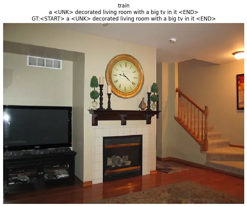
Train에서는 small-data에 overfitting시켰기 때문에 ground-truth(correct label)와 동일한 caption을 생성하는 모습이 보인다.

반면 validation에서는 문법이 자연스럽지 않고, 사람과 주변 배경 등 이미지의 전반적인 구조도 제대로 포착하지 못하는 모습이 보인다.
Vision Transformer (ViT)
Vision Transformer(ViT)는 이미지를 여러 개의 patch로 나누고, 각 patch를 하나의 token처럼 임베딩하여 Transformer encoder에 입력하는 모델이다.
이미지는 patch embedding을 통해 다음과 같은 형태의 시퀀스로 변환된다.
이후 positional encoding을 추가하여 각 patch의 위치 정보를 보존하고, Transformer encoder를 통해 patch들 사이의 관계를 학습한다.
최종적으로 Transformer의 출력 representation을 이용하여 이미지 분류 등의 작업을 수행한다.
Patch Embedding
class PatchEmbedding(nn.Module):
    """
    A layer that splits an image into patches and projects each patch to an embedding vector.
    Used as the input layer of a Vision Transformer (ViT).

    Inputs:
    - img_size: Integer representing the height/width of input image (assumes square image).
    - patch_size: Integer representing height/width of each patch (square patch).
    - in_channels: Number of input image channels (e.g., 3 for RGB).
    - embed_dim: Dimension of the linear embedding space.
    """
    def __init__(self, img_size, patch_size, in_channels=3, embed_dim=128):
        super().__init__()

        self.img_size = img_size
        self.patch_size = patch_size
        self.in_channels = in_channels
        self.embed_dim = embed_dim

        assert img_size % patch_size == 0, "Image dimensions must be divisible by the patch size."

        self.num_patches = (img_size // patch_size) ** 2
        self.patch_dim = patch_size * patch_size * in_channels

        # Linear projection of flattened patches to the embedding dimension
        self.proj = nn.Linear(self.patch_dim, embed_dim)


    def forward(self, x):
        """
        Forward pass for patch embedding.

        Inputs:
        - x: Input image tensor of shape (N, C, H, W)

        Returns:
        - out: Patch embeddings with shape (N, num_patches, embed_dim)
        """
        N, C, H, W = x.shape
        assert H == self.img_size and W == self.img_size, \
            f"Expected image size ({self.img_size}, {self.img_size}), but got ({H}, {W})"
        out = torch.zeros(N, self.embed_dim)

        """
        차원 계산
        goal: (N, num_patches, patch_dim)
        image_size = H == W
        num_patches = (image_size // patch_size)**2
                    = (H // patch_size)(W // patch_size)
        patch_dim = patch_size * patch_size * C
        """

        P = self.patch_size

        x_convert = x.reshape(N, C, H//P, P, W//P, P) # (0, 1, 2, 3, 4, 5)
        x_convert = x_convert.permute(0, 2, 4, 1, 3, 5) # (N, H//P, W//P, C, P, P)
        x_convert = x_convert.reshape(N, H//P * W//P, C * P * P) # (N, num_patches, patch_dim)

        # (N, num_patches, patch_dim) @ (patch_dim, embed_dim) -> (N, num_patches, embed_dim)
        out = self.proj(x_convert)

        return out
TransformerEncoderLayer
각 patch token은 self-attention으로 다른 patch의 정보를 받아오고, FFN으로 각 token의 feature를 변환한다. 두 sublayer 모두 residual connection과 dropout, LayerNorm을 거치며 입출력 shape은 로 유지된다.
class TransformerEncoderLayer(nn.Module):
    """
    A single layer of a Transformer encoder, to be used with TransformerEncoder.
    """
    def __init__(self, input_dim, num_heads, dim_feedforward=2048, dropout=0.1):
        """
        Construct a TransformerEncoderLayer instance.

        Inputs:
         - input_dim: Number of expected features in the input.
         - num_heads: Number of attention heads.
         - dim_feedforward: Dimension of the feedforward network model.
         - dropout: The dropout value.
        """
        super().__init__()
        self.self_attn = MultiHeadAttention(input_dim, num_heads, dropout)
        self.ffn = FeedForwardNetwork(input_dim, dim_feedforward, dropout)

        self.norm_self = nn.LayerNorm(input_dim)
        self.norm_ffn = nn.LayerNorm(input_dim)

        self.dropout_self = nn.Dropout(dropout)
        self.dropout_ffn = nn.Dropout(dropout)

    def forward(self, src, src_mask=None):
        """
        Pass the inputs (and mask) through the encoder layer.

        Inputs:
        - src: the sequence to the encoder layer, of shape (N, S, D)
        - src_mask: the parts of the source sequence to mask, of shape (S, S)

        Returns:
        - out: the Transformer features, of shape (N, S, D)
        """

        # (N, S, D) -> (N, S, D)
        # Self-Attention -> Dropout -> Residual Conn -> LayerNorm
        shortcut = src
        self_attn_out = self.self_attn(query=src, key=src, value=src, attn_mask=src_mask)
        self_attn_out = self.dropout_self(self_attn_out)
        src = self_attn_out + shortcut
        src = self.norm_self(src)

        # FFN -> Dropout -> Residual Conn -> LayerNorm
        shortcut = src
        src = self.ffn(src)
        src = self.dropout_ffn(src)
        src = src + shortcut
        src = self.norm_ffn(src)

        return src
Vision Transformer
이미지를 patch token으로 변환하고 positional encoding을 더한 뒤 여러 Transformer encoder layer를 통과시킨다. 마지막에는 patch token 전체를 평균 내어 하나의 image representation을 만들고, linear head로 class score를 계산한다.
patch token들의 평균을 구하는 이유는 최종 분류에서 이미지 한 장당 클래스 하나를 예측해야 하니까, patch P개를 이미지 전체를 대표하는 하나의 벡터로 합쳐야 하기 때문이다.
class VisionTransformer(nn.Module):
    """
    Vision Transformer (ViT) implementation.
    """
    def __init__(self, img_size=32, patch_size=8, in_channels=3,
                 embed_dim=128, num_layers=6, num_heads=4,
                 dim_feedforward=256, num_classes=10, dropout=0.1):
        """
        Inputs:
         - img_size: Size of input image (assumed square).
         - patch_size: Size of each patch (assumed square).
         - in_channels: Number of image channels.
         - embed_dim: Embedding dimension for each patch.
         - num_layers: Number of Transformer encoder layers.
         - num_heads: Number of attention heads.
         - dim_feedforward: Hidden size of feedforward network.
         - num_classes: Number of classification labels.
         - dropout: Dropout probability.
        """
        super().__init__()
        self.num_classes = num_classes
        self.patch_embed = PatchEmbedding(img_size, patch_size, in_channels, embed_dim)
        self.positional_encoding = PositionalEncoding(embed_dim, dropout=dropout)

        encoder_layer = TransformerEncoderLayer(embed_dim, num_heads, dim_feedforward, dropout)
        self.transformer = TransformerEncoder(encoder_layer, num_layers=num_layers)

        # Final classification layer to predict class scores from pooled token.
        self.head = nn.Linear(embed_dim, num_classes)

        self.apply(self._init_weights)


    def _init_weights(self, module):
        """
        Initialize the weights of the network.
        """
        if isinstance(module, (nn.Linear, nn.Embedding)):
            module.weight.data.normal_(mean=0.0, std=0.02)
            if isinstance(module, nn.Linear) and module.bias is not None:
                module.bias.data.zero_()
        elif isinstance(module, nn.LayerNorm):
            module.bias.data.zero_()
            module.weight.data.fill_(1.0)

    def forward(self, x):
        """
        Forward pass of Vision Transformer.

        Inputs:
         - x: Input image tensor of shape (N, C, H, W)

        Returns:
         - logits: Output classification logits of shape (N, num_classes)
        """
        N = x.size(0)
        logits = torch.zeros(N, self.num_classes, device=x.device)

        # (N, P, E)
        x = self.patch_embed(x)
        x = self.positional_encoding(x)
        # (N, P, E)
        x = self.transformer(x)
        # (N, E)
        x_mean = x.mean(dim=1)
        logits = self.head(x_mean)


        return logits
추가 개념들
Vision Transformer 학습 결과
learning_rate = 1e-3
weight_decay = 0.0
batch_size = 64

model = VisionTransformer(
    img_size=32,
    patch_size=4,
    in_channels=3,
    embed_dim=128,
    num_layers=4,
    num_heads=4,
    dim_feedforward=256,
    num_classes=10,
    dropout=0.1,
)
CIFAR-10의 입력 이미지는 로 크기가 작기 때문에, 너무 큰 patch를 사용하면 하나의 patch에 많은 공간 정보가 압축되어 세부적인 특징을 잃을 수 있다고 생각했다. 따라서 patch_size=4로 설정하여 하나의 패치가 CNN의 작은 커널처럼 특정한 공간 정보를 잡을 수 있게 했다.
이 경우 한 이미지에서 생성되는 patch의 개수는 다음과 같다.
따라서 이미지는 64개의 patch token으로 변환되어 Transformer에 입력된다.
학습률은 1e-4로 설정하였다. Adam optimizer를 사용하는 상황에서 너무 큰 학습률로 인해 학습이 불안정해지는 것을 방지하면서, 안정적으로 loss가 감소하도록 비교적 작은 학습률을 사용하였다.
weight_decay 는 0.0으로 설정하여 weight decay에 의한 추가적인 정규화를 적용하지 않았다. 이번 과제는 2 epoch이라는 짧은 학습 시간 안에 충분한 학습 성능을 얻는 것이 목표이므로, 가중치 크기를 억제하는 것보다 학습 데이터에 빠르게 적합하도록 하는 것을 우선하였다.

위 설정으로 2 epoch 학습한 결과 train과 test loss가 모두 감소했으며, 최종 test accuracy는 로 약 를 기록했다.
Inline Question 1
Several key design decisions were made in designing the scaled dot-product attention introduced above. Explain why the following choices were beneficial:
- Using multiple attention heads as opposed to one.
- Dividing by before applying the softmax function. Recall that is the feature dimension and is the number of heads.
- Adding a linear transformation to the output of the attention operation.
Only one or two sentences per choice are necessary, but be specific about what would happen without each implementation detail, why that would be suboptimal, and how the proposed implementation improves the situation.
Your Answer:
- Multiple attention heads
Multiple attention heads allow the model to view the same input from different perspectives and capture relationships in different representation subspaces. With only one head, all relationships would need to be represented by a single attention pattern.
여러개의 어텐션 헤드를 통해 같은 입력을 서로 다른 관점에서 볼 수 있게 된다. 다양한 표현공간에서 입력을 판단할 수 있게 된다.
- Scaled dot-product scores
Dividing the dot-product scores by the square root of the per-head dimension, , keeps their variance under control as the head dimension grows. Without this scaling, softmax could saturate and produce very small gradients; scaling stabilizes both the scores and gradient flow.
dot-product score 를 각 헤드 차원 로 나눠줌으로써 각 결과의 분산을 낮춰 softmax가 안정적으로 수행될 수 있게 한다. 헤드차원 가 커질수록 소프트맥스가 포화될 수 있으므로, 스케일링으로 score 크기를 안정화하고 gradient vanishing 을 막는다.
- Output linear transformation
Simply concatenating the head outputs leaves the information from each head separated. The output linear transformation learns how to mix information across heads into a unified final representation.
각 head의 출력을 단순히 concatenate하면 head별 정보가 서로 분리되어 있다. Output linear transformation은 여러 head의 정보를 학습 가능한 방식으로 섞어 최종 representation을 만든다.
Inline Question 2
Despite their recent success in large-scale image recognition tasks, ViTs often lag behind traditional CNNs when trained on smaller datasets. What underlying factors contribute to this performance gap? What techniques can be used to improve the performance of ViTs on small datasets?
Your Answer:
On small datasets, CNNs often outperform ViTs because convolution provides strong image-specific inductive biases. A convolutional layer extracts local features and shares the same kernel across the entire image, so it can learn useful spatial features from relatively little data.
In contrast, a ViT converts an image into a sequence of patches and uses self-attention to learn the relationships between them. Since it makes weaker assumptions about image structure, such as locality, it must learn these relationships directly from data and can therefore be at a disadvantage when the dataset is small.
ViT performance on small datasets can be improved through data augmentation, which exposes the model to more varied inputs, or through transfer learning by fine-tuning a ViT pretrained on a large image dataset. Regularization can also reduce overfitting to the small training set.
작은 데이터셋에서는 CNN이 ViT보다 좋은 성능을 보이는 경우가 많다. CNN은 convolution 을 통해서 국소 특징을 추출하고, 동일한 kernel을 이미지 전체에 공유하는 구조를 가지므로, 이미지의 공간적 특성에 대한 inductive bias가 모델 레벨에서 강하다. 따라서 비교적 적은 데이터만으로도 유용한 특징을 학습할 수 있다. 반면 ViT는 이미지를 patch sequence로 변환한 뒤 self-attention을 이용하여 patch 사이의 관계를 학습한다. CNN에 비해 이미지의 locality와 같은 구조적 가정이 약하기 때문에 이러한 관계를 데이터로부터 직접 학습해야 하며, 작은 데이터셋에서는 상대적으로 불리할 수 있다.
작은 데이터셋에서 ViT의 성능을 향상시키기 위해서는 data argumentation 등으로 제한된 데이터셋에서 더 다양한 입력을 제공하여 가능한 많은 관계를 학습하도록 유도할 수 있다. 또는 일반적인 대규모 이미지모델에서 학습된 ViT를 베이스로 사용하고, 작은 데이터셋에서 추가적인 fine-turning을 수행하는 transfer learning을 이용하면 적은 데이터만으로도 더 나은 성능을 기대해 볼 수 있다. 또한 regulazation을 이용하여 작은 데이터셋에 overfitting 되는 문제점도 완화 가능하다.
Inline Question 3
How does the computational cost of the self-attention layers in a ViT change if we independently make the following changes? Please ignore the computation cost of QKV and output projection.
(i) Double the hidden dimension.
(ii) Double the height and width of the input image.
(iii) Double the patch size.
(iv) Double the number of layers.
Your Answer:
Ignoring the QKV and output projections, the matrix multiplications and each have a computational cost of , where is the number of patch tokens and is the hidden dimension.
-
When the hidden dimension is doubled, the cost of changes from to . Since a general matrix multiplication costs , self-attention is quadratic in the sequence length but linear in the hidden dimension. The cost therefore doubles.
-
If both the height and width of the input image are doubled while the patch size remains fixed, the number of patches becomes four times larger. The attention input then contains patch tokens, so the cost becomes , which is 16 times the original cost.
-
If the patch size is doubled along both spatial dimensions, the number of patches becomes one quarter of the original: . The attention cost becomes , so it decreases to of the original cost.
-
If the number of self-attention layers is doubled, each layer still performs and . These operations are therefore performed twice as many times, so the total self-attention cost doubles.
QKV projection 및 output projection을 제외 했을때, 1. matmul을 수행할 때 hidden dimension이 두 배가 되면 행렬곱의 연산량도 두 배로 증가한다. 기존 연산량은 이고, hidden dimension이 두 배가 되면 가 된다. 일반적인 행렬곱의 연산량이 이므로, self-attention은 sequence에 대해서는 quadratic하지만 hidden dimension에 대해서는 선형적으로 증가한다. 따라서 hidden dimension을 두 배로 하면 해당 연산량도 두 배가 된다.
2.입력 이미지의 높이와 너비가 두배가 되는 경우, 같은 patch size P를 고정할 경우 patch embedding 과정에서 patch의 갯수가 4배가 되고, 셀프 어텐션 입력으로 (N, 4P, )이 주어지므로 self-attention 시 계산량은 대략 이므로 계산량이 16배로 증가한다.
3.patch size가 두배가 된 경우, patch 개수는 1/4로 감소하고(P=(H/2p)(W/2p)), 어텐션 입력으로 (N, 1/4P, ) 이 주어지므로 다음 행렬 곱셈 시 계산량은 대략 이므로 기존의 1/16까지 계산량이 감소한다.
4.self-attention layer의 개수가 두 배로 증가하면 각 layer에서 수행되는 와 연산도 두 배의 횟수로 수행되므로, 전체 self-attention 계산량은 두 배로 증가한다.