핵심 한 줄 정리

Image segmentation과 object detection은 image-level classification을 pixel, region, object 단위의 dense prediction으로 확장한 문제이며, saliency map과 CAM(Class Activation Mapping) 계열 기법은 예측 score를 다시 image 공간에 연결해 model이 어느 영역을 사용했는지 해석한다.

중요 개념 정리

Computer vision task의 출력 단위

같은 image를 입력받더라도 무엇을 출력하느냐에 따라 task가 달라진다.

Task	출력	같은 class의 여러 object 구분
Image classification	image 전체의 class 하나	불가능
Semantic segmentation	pixel마다 semantic class	불가능
Object detection	object마다 class와 bounding box	가능
Instance segmentation	object마다 class, box, pixel mask	가능

Semantic segmentation에서 dog가 두 마리 있으면 두 object의 pixel은 모두 dog class로 표시된다. Instance segmentation은 같은 dog class 안에서도 서로 다른 instance ID를 부여한다.

이 task들은 입력 image 하나를 label 하나로 줄이는 classification보다 출력 구조가 복잡하다. Spatial information을 유지하면서 image의 여러 위치에 prediction을 만들어야 하므로 dense prediction이라고 부른다.

Semantic segmentation

Semantic segmentation은 image의 모든 pixel에 class label을 할당하는 문제이다.

Input image가 다음 shape라고 하자.

$$X \in \mathbb{R}^{H \times W \times C_{\text{in}}}$$

Class 수가 $K$이면 model은 pixel마다 $K$개의 score를 출력한다.

$$S \in \mathbb{R}^{H \times W \times K}$$

최종 segmentation map은 각 pixel에서 score가 가장 큰 class를 선택한다.

$$\hat{y}_{i,j} = \arg\max_{k}S_{i,j,k}$$

Pixel 하나의 RGB(Red, Green, Blue) 값만 보고 class를 결정하기는 어렵다. 같은 색도 object와 주변 context에 따라 의미가 달라지므로 model의 receptive field가 주변 영역을 함께 봐야 한다.

각 pixel을 중심으로 patch를 잘라 image classifier를 반복 실행할 수도 있지만, $H \times W$개의 pixel마다 full network를 실행하므로 계산이 지나치게 크다. 실제로는 image 전체를 한 번 입력해 모든 pixel의 prediction을 동시에 만든다.

FCN(Fully Convolutional Network)

FCN은 fully connected layer를 사용하지 않고 convolutional layer만으로 spatial output을 생성한다. Input resolution을 줄이는 encoder와 다시 키우는 decoder로 구성할 수 있다.

$$H \times W \xrightarrow{\text{encoder}} h \times w \xrightarrow{\text{decoder}} H \times W$$

Encoder는 pooling이나 strided convolution으로 resolution을 줄인다. Resolution이 작아질수록 계산량이 줄고 receptive field가 커지며, channel 수를 늘려 더 추상적인 feature를 저장한다.

$$H,W \downarrow \qquad C \uparrow$$

Decoder는 low-resolution feature map을 원래 image resolution으로 upsampling한다. 마지막 $1 \times 1$ convolution은 각 위치의 feature vector를 $K$개의 class score로 바꾼다.

$$F_{i,j} \in \mathbb{R}^{C} \xrightarrow{1 \times 1\text{ Conv}} S_{i,j} \in \mathbb{R}^{K}$$

Pixel-wise classification loss

Semantic segmentation은 모든 pixel에서 classification을 수행한다. Ground-truth label map을 $Y \in \{1,\ldots,K\}^{H \times W}$라고 하면 pixel-wise cross-entropy loss는 다음과 같다.

$$L_{i,j} = -\log \frac{\exp(S_{i,j,Y_{i,j}})} {\sum_{k=1}^{K}\exp(S_{i,j,k})}$$

Image 전체의 loss는 유효한 pixel의 loss를 합하거나 평균 낸 값이다.

$$L_{\text{seg}} = \frac{1}{|\Omega|} \sum_{(i,j)\in\Omega}L_{i,j}$$

$\Omega$는 annotation이 있는 유효 pixel 집합이다. Fully supervised segmentation은 pixel-level ground-truth map이 필요하며, 초기 dataset은 사람이 각 pixel을 직접 표시해 만들었다.

Class별 pixel 수가 크게 다르면 background가 loss를 지배할 수 있다. 이때 class weight를 적용하거나 focal loss, Dice loss 같은 대안을 사용할 수 있다.

Upsampling

Downsampling은 pooling이나 stride로 쉽게 수행할 수 있지만 decoder에는 resolution을 키우는 연산이 필요하다.

Nearest-neighbor upsampling

Nearest-neighbor upsampling은 low-resolution 값을 주변 위치에 그대로 복사한다. $2 \times 2$ feature map을 scale factor 2로 키우면 $4 \times 4$가 된다.

$$\begin{bmatrix} a & b \\ c & d \end{bmatrix} \longrightarrow \begin{bmatrix} a & a & b & b \\ a & a & b & b \\ c & c & d & d \\ c & c & d & d \end{bmatrix}$$

학습 parameter가 없으며, 보통 뒤에 convolution을 붙여 feature를 보정한다.

Bed-of-nails upsampling

Bed-of-nails 방식은 정해진 위치에 원래 값을 놓고 나머지를 $0$으로 채운다.

$$\begin{bmatrix} a & b \\ c & d \end{bmatrix} \longrightarrow \begin{bmatrix} a & 0 & b & 0 \\ 0 & 0 & 0 & 0 \\ c & 0 & d & 0 \\ 0 & 0 & 0 & 0 \end{bmatrix}$$

뒤쪽 convolution이 비어 있는 위치로 정보를 퍼뜨린다.

Max unpooling

Encoder에서 max pooling을 수행할 때 선택된 maximum의 위치를 저장해 두었다가 decoder에서 같은 위치에 값을 되돌릴 수 있다. 저장한 argmax index가 spatial structure를 복원하는 힌트가 된다.

Max unpooling도 학습 parameter가 없는 연산이며, pooling에서 버린 정확한 값까지 복구하는 것은 아니다.

Transposed convolution

Transposed convolution은 학습 가능한 upsampling 연산이다. Input의 각 값을 kernel로 펼쳐 output 위치에 더하며, overlap되는 위치는 합산한다.

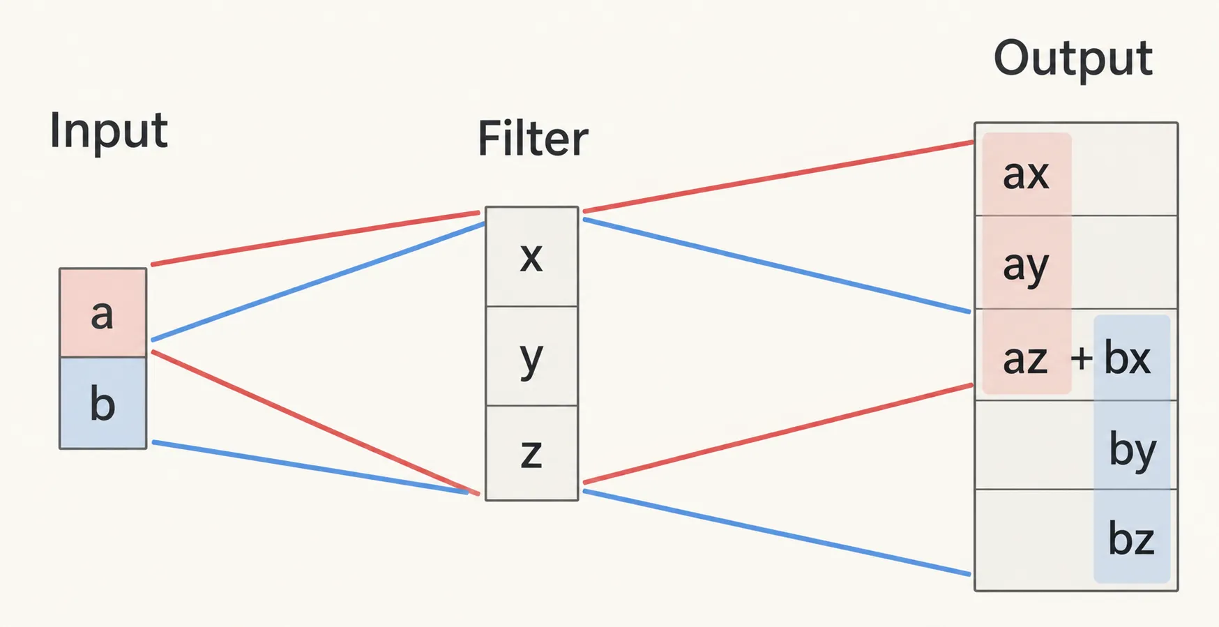
1차원에서 input이 $[A,B]$이고 kernel이 $[w_1,w_2,w_3]$이면 stride 1의 output은 다음과 같은 형태가 된다.

$$[A,B] \longrightarrow [Aw_1,Aw_2+Bw_1,Aw_3+Bw_2,Bw_3]$$

2차원 output size는 kernel size $K$, stride $S$, padding $P$, output padding $P_{\text{out}}$에 따라 다음처럼 계산한다.

$$H_{\text{out}} = (H_{\text{in}}-1)S-2P+K+P_{\text{out}}$$

Transposed convolution이라는 이름은 convolution을 matrix multiplication으로 표현했을 때 그 matrix의 transpose를 사용하는 데서 나온다. 일반 convolution의 정보를 정확히 되돌리는 inverse convolution은 아니다.

U-Net

U-Net은 encoder-decoder 구조에 같은 resolution끼리 연결하는 skip connection을 추가한 segmentation network이다.

$$F_{\text{dec}}^{(l)} = \operatorname{Concat} \left( \operatorname{Upsample}(F_{\text{dec}}^{(l+1)}), F_{\text{enc}}^{(l)} \right)$$

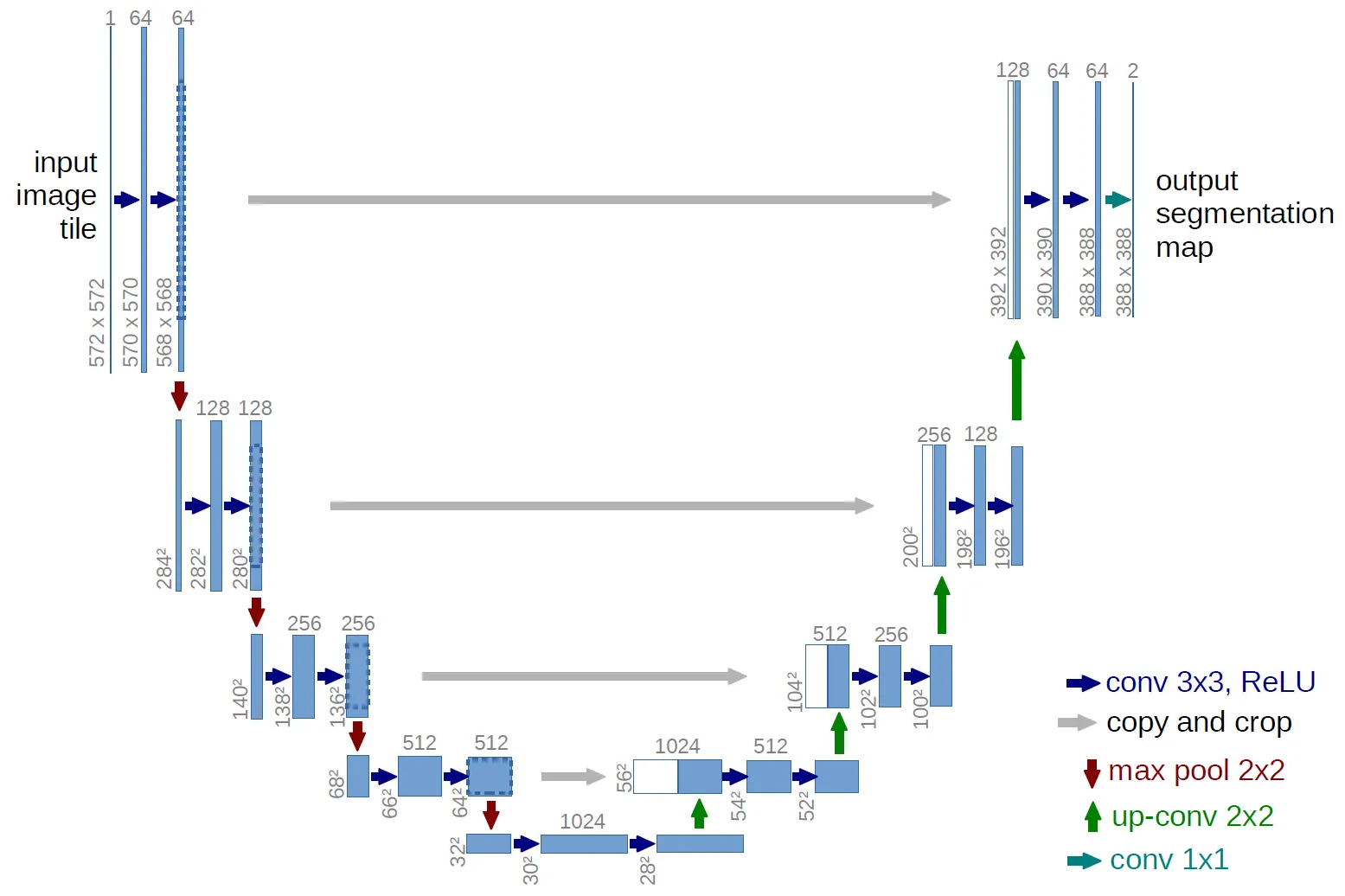Encoder의 깊은 feature는 넓은 context와 semantic information을 담지만 downsampling 과정에서 정확한 boundary와 위치 정보가 약해진다. 같은 resolution의 encoder feature를 decoder에 직접 전달하면 다음 두 정보를 함께 사용할 수 있다.

• 깊은 layer의 semantic context
• 얕은 layer의 세밀한 spatial structure

이 skip connection 덕분에 object boundary가 더 선명한 segmentation map을 만들 수 있다. U-Net과 그 변형은 medical image segmentation처럼 pixel 위치가 중요한 task에서 여전히 강한 baseline이다.

%% title: U-Net Encoder-Decoder와 Skip Connection
%% caption: 256 × 256 input을 예로 든 U-Net이다. Encoder는 해상도를 절반으로 줄이며 채널을 늘리고, decoder는 같은 해상도의 encoder feature를 concatenate해 경계 정보를 복원한다.
flowchart LR
    image["Image<br/>3 × 256 × 256"] --> e1["Encoder Conv Block 1<br/>64 × 256 × 256"]
    e1 -->|"MaxPool /2"| e2["Encoder Conv Block 2<br/>128 × 128 × 128"]
    e2 -->|"MaxPool /2"| bottleneck["Bottleneck<br/>256 × 64 × 64"]
    bottleneck -->|"Upsample ×2"| d2["Decoder Conv Block 2<br/>128 × 128 × 128"]
    d2 -->|"Upsample ×2"| d1["Decoder Conv Block 1<br/>64 × 256 × 256"]
    d1 --> mask["1 × 1 Conv<br/>K × 256 × 256"]
    e2 -. "skip: concat" .-> d2
    e1 -. "skip: concat" .-> d1

Semantic segmentation과 instance segmentation

Semantic segmentation output은 class별 map이다.

$$Y_{\text{semantic}} \in \{1,\ldots,K\}^{H \times W}$$

같은 class object가 여러 개 있어도 하나의 class ID만 표시되므로 서로 다른 instance를 구분할 수 없다. Instance segmentation은 각 object를 먼저 분리하고 object마다 binary mask를 예측한다.

$$\mathcal{O} = \left\{ (c_n,b_n,m_n) \right\}_{n=1}^{N}$$

$c_n$은 class, $b_n$은 bounding box, $m_n$은 해당 instance의 mask이다. 따라서 instance segmentation은 object detection과 pixel segmentation을 결합한 task로 볼 수 있다.

Object detection의 출력

Object detection은 image 안의 각 object에 대해 class와 bounding box를 예측한다.

$$\mathcal{D} = \left\{ (p_n,b_n) \right\}_{n=1}^{N}$$

$p_n$은 class probability vector이고 bounding box는 예를 들어 다음 네 값으로 표현할 수 있다.

$$b_n = (x_n,y_n,w_n,h_n)$$

Single-object image라면 network가 class score와 box coordinate 네 개를 직접 출력할 수 있다. Loss는 classification과 box regression을 합한 multi-task loss이다.

$$L = L_{\text{cls}} + \lambda L_{\text{box}}$$

강의의 단순한 설정에서는 class에 softmax loss, box coordinate에 L2 loss를 사용한다.

$$L_{\text{box}} = \lVert b-\hat{b}\rVert_2^2$$

실제 detector에서는 outlier에 덜 민감한 Smooth L1 loss나 box overlap을 직접 반영하는 loss도 자주 사용한다.

Object 수 $N$은 image마다 다르다. Object가 세 개라면 box coordinate만 $12$개가 필요하고 object 수가 바뀌면 output 길이도 달라진다. 고정된 output vector에 모든 object를 단순히 나열하는 방식은 확장하기 어렵다.

IoU(Intersection over Union)

Detection에서 predicted box와 ground-truth box가 얼마나 겹치는지는 IoU로 측정한다.

$$\operatorname{IoU}(B_p,B_g) = \frac{|B_p\cap B_g|}{|B_p\cup B_g|}$$

두 box가 완전히 같으면 IoU는 $1$, 전혀 겹치지 않으면 $0$이다. 일정 IoU threshold 이상이면서 class도 맞아야 true positive로 판단한다.

Detection 성능은 confidence threshold를 바꾸며 precision과 recall을 계산해 평가한다. Precision은 model이 검출했다고 판단한 결과 중 실제 object를 올바르게 찾은 비율이고, recall은 실제 존재하는 object 중 model이 찾아낸 비율이다.

TP(True Positive)는 올바른 detection, FP(False Positive)는 잘못된 detection, FN(False Negative)는 놓친 object를 뜻한다.

$$\operatorname{Precision} = \frac{TP}{TP+FP} \qquad \operatorname{Recall} = \frac{TP}{TP+FN}$$

Precision-Recall curve는 confidence threshold를 바꾸며 얻은 recall을 가로축, precision을 세로축에 나타낸 곡선이다. Threshold를 낮추면 더 많은 object를 검출해 recall은 높아지지만 false positive도 늘어 precision이 낮아질 수 있으며, 이 곡선은 두 지표 사이의 trade-off를 보여준다.

Precision-Recall curve 아래 면적은 AP(Average Precision)로 요약한다. 여러 class의 AP를 평균 낸 값은 mAP(mean Average Precision)이다.

$$\operatorname{mAP} = \frac{1}{K} \sum_{k=1}^{K}\operatorname{AP}_k$$

Dataset에 따라 IoU $0.5$ 한 지점의 AP를 쓰거나, $0.50$부터 $0.95$까지 여러 threshold의 AP를 평균 내기도 한다.

Sliding window와 region proposal

고정된 window를 image 전체의 여러 위치와 scale에 옮기며 각 crop을 object class 또는 background로 분류할 수 있다. 그러나 $(x,y,w,h)$의 가능한 조합이 너무 많아 모든 window에 CNN(Convolutional Neural Network)을 실행하는 것은 비효율적이다.

Region proposal은 object가 있을 가능성이 높은 소수의 후보 box만 먼저 선택한다. Detector는 각 proposal에 대해 다음 두 task를 수행한다.

• proposal 안의 object class를 분류한다.
• ground-truth box에 더 잘 맞도록 coordinate offset을 예측한다.

$$\hat{b} = b_{\text{proposal}}+\Delta b$$

Region proposal 기반 detector는 detection 문제를 제한된 수의 region classification과 box refinement 문제로 바꾼다.

R-CNN(Region-based Convolutional Neural Network) 계열

R-CNN

R-CNN은 image에서 region proposal을 만든 뒤 각 region을 crop하고 독립적으로 CNN에 통과시킨다.

$$\text{Image} \rightarrow \text{Region proposals} \rightarrow \text{CNN per region} \rightarrow \text{Class + Box offset}$$

같은 image의 겹치는 region마다 CNN computation을 반복하므로 매우 느리다.

Fast R-CNN

Fast R-CNN은 CNN을 image 전체에 한 번만 적용한다. Proposal을 image가 아니라 shared feature map에 투영하고, 각 region의 feature를 ROI(Region of Interest) pooling으로 고정된 크기로 바꾼 뒤 class와 box offset을 예측한다.

$$\text{Image} \xrightarrow{\text{CNN once}} F \xrightarrow{\text{ROI features}} \text{Class + Box offset}$$

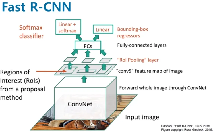
Convolution feature map이 spatial correspondence를 유지하므로 image의 proposal 위치를 feature map 위치로 옮길 수 있다. R-CNN의 중복 convolution을 제거한 것이 핵심이다.

Faster R-CNN과 RPN(Region Proposal Network)

Faster R-CNN은 별도 proposal algorithm 대신 RPN을 feature map 위에서 학습한다. 여러 위치와 scale의 anchor마다 다음 값을 예측한다.

• object가 있을 확률인 objectness score
• anchor를 object box에 맞추는 coordinate offset

Confidence가 높은 top $K$ proposal을 선택해 두 번째 detection head로 보낸다. 따라서 Faster R-CNN은 다음 두 stage로 구성된다.

1. RPN이 object candidate를 만든다.
2. Detection head가 proposal의 class와 box를 정교하게 예측한다.

Two-stage detector는 정확도가 높지만 proposal과 detection을 나누어 처리하므로 one-stage detector보다 latency가 커질 수 있다.

Faster-R-CNN 구조 참고_wikidocs

One-stage detector와 YOLO(You Only Look Once)

One-stage detector는 별도의 region proposal 단계를 두지 않고, 하나의 network에서 bounding box와 class를 직접 예측한다. SSD(Single Shot MultiBox Detector)와 YOLO가 대표적이다. (SSD 논문, YOLOv1 논문)

YOLO는 이미지를 S×S grid로 나누고, 모든 grid cell의 prediction을 한 번의 forward pass에서 함께 생성한다.

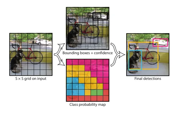
각 grid cell은 B개의 bounding box를 예측한다. 이때 bounding box의 중심은 해당 cell을 기준으로 표현되지만, box의 크기는 cell 영역에 제한되지 않으므로 여러 grid cell에 걸쳐 확장될 수 있다.

각 grid cell은 각 box의 confidence와 cell당 한 세트의 K개 conditional class probability도 함께 예측한다.

강의와 YOLOv1 논문의 예시에서는 다음 값을 사용한다.

$$S=7, \qquad B=2$$

각 grid cell이 두 개의 candidate bounding box를 예측하므로 image 전체에서 나오는 bounding box 후보 수는 다음과 같다.

$$7\times7\times2=98$$

Grid cell 하나의 output 크기는 다음과 같다.

$$\text{output per cell} = B\times(4+1)+K$$

Output vector의 각 위치가 갖는 역할

한 grid cell에서 B=2, K=3이라고 하자. 이 cell의 output vector는 다음과 같이 각 위치의 역할이 미리 정해져 있다.

[
  x1, y1, w1, h1, conf1,  # bounding box 1
  x2, y2, w2, h2, conf2,  # bounding box 2
  p1, p2, p3              # cell의 class probability
]

Network는 처음에는 단지 $13$개의 숫자를 출력한다. 각 위치에 bounding box coordinate, confidence, class probability라는 의미를 부여하는 것은 loss이다. 학습할 때 각 위치를 서로 다른 ground-truth target과 비교하므로 output마다 서로 다른 gradient가 발생한다.

각 bounding box는 네 개의 coordinate와 하나의 confidence를 가진다.

$$(x,y,w,h,\text{confidence})$$

YOLOv1의 confidence는 단순한 object probability가 아니라 object의 존재 여부와 predicted box의 IoU를 함께 반영한 값이다.

$$\text{confidence} = P(\text{Object}) \times \operatorname{IoU}$$

$K$개의 class probability는 bounding box마다 따로 붙는 값이 아니라 grid cell마다 한 세트만 예측한다.

Responsible cell과 responsible predictor

학습할 때는 GT(Ground Truth) object의 중심이 들어 있는 grid cell을 해당 object의 responsible cell로 정한다. 이는 그 object의 위치와 class를 맞게 예측하도록 loss를 부여받은 cell이다.

Responsible cell 안에서도 $B$개의 predicted box 중 ground-truth box와 IoU가 가장 높은 하나를 responsible predictor로 정한다.

bounding box 1 ── IoU = 0.25
bounding box 2 ── IoU = 0.73  ← responsible predictor

Responsible predictor에는 coordinate와 object가 있는 경우의 confidence loss를 적용한다. 나머지 predictor에는 coordinate loss를 적용하지 않고, confidence를 낮추는 loss를 적용한다. Class loss는 bounding box마다 계산하지 않고 object가 있는 responsible cell에 한 번 적용한다.

bounding box 1
├─ coordinate loss: 적용하지 않음
└─ confidence loss: 0을 향하도록 적용

bounding box 2
├─ x, y, w, h coordinate loss
└─ confidence loss: ground-truth와의 IoU를 향하도록 적용

grid cell
└─ class loss: ground-truth class를 향하도록 적용

Responsible cell과 predictor를 정하는 과정은 object를 발견한 뒤 해당 위치에서 prediction을 다시 수행한다는 뜻이 아니다. 모든 cell의 prediction은 이미 한 번에 계산되어 있으며, ground-truth object를 어느 output과 비교해 학습시킬지를 정하는 training rule이다.

Coordinate, confidence, class의 학습

Bounding box coordinate

Responsible predictor의 coordinate와 ground-truth coordinate를 비교한다. 가장 단순한 형태로 나타내면 다음과 같다.

$$L_{\text{coord}}^{\text{simple}} = (\hat{x}-x)^2 +(\hat{y}-y)^2 +(\hat{w}-w)^2 +(\hat{h}-h)^2$$

예측한 중심의 $x$ coordinate가 실제 값과 다르면 해당 output에는 다음 gradient가 발생한다.

$$\frac{\partial L}{\partial \hat{x}} = 2(\hat{x}-x)$$

이 gradient가 shared CNN까지 전달되면서 visual feature와 coordinate를 연결하는 parameter가 바뀐다. 사람이 object boundary를 찾는 rule을 직접 넣는 것이 아니라, 여러 image의 coordinate loss를 줄이는 방향으로 network가 box 위치와 크기를 학습한다.

Confidence

Confidence도 target과의 차이로 학습한다. 개념적으로는 다음과 같이 나타낼 수 있다.

$$L_{\text{conf}} = (\hat{C}-C)^2$$

Responsible predictor의 target $C$는 predicted box와 ground-truth box의 IoU이고, object가 없는 cell과 responsible predictor가 아닌 box의 target은 $0$이다. 따라서 빈 영역에서 높은 confidence를 출력하면 이를 낮추는 방향으로 gradient가 발생한다.

Class probability

Object가 있는 cell에는 ground-truth class를 target으로 사용한다. Class가 cat, dog, car이고 정답이 dog이라면 target은 다음과 같다.

$$[0,1,0]$$

Prediction이 $[0.6,0.2,0.2]$라면 dog에 해당하는 값을 높이고 나머지를 낮추는 방향으로 gradient가 전달된다. 이 class loss는 cell당 한 세트의 class probability에 적용된다.

전체 loss와 backpropagation

YOLOv1의 전체 loss는 coordinate, confidence, class loss를 하나의 scalar로 합친다. 간략히 나타내면 다음과 같다.

$$L = \lambda_{\text{coord}}L_{\text{coord}} +L_{\text{conf,obj}} +\lambda_{\text{noobj}}L_{\text{conf,noobj}} +L_{\text{class}}$$

실제 coordinate loss는 width와 height에 square root를 적용해 큰 box와 작은 box의 오차가 균형 있게 반영되도록 한다. Object가 없는 경우의 confidence loss에는 별도의 weight를 두어 빈 cell이 전체 loss를 지배하지 않게 한다.

image
  ↓
shared CNN feature
  ↓
역할이 정해진 grid output
  ├─ bounding box coordinate loss
  ├─ confidence loss
  └─ class loss
          ↓
      total loss
          ↓
    backpropagation
          ↓
CNN 전체 parameter update

앞부분의 CNN feature는 coordinate, confidence, class prediction에 공통으로 사용된다. 따라서 같은 feature가 object가 어디에 있는지, object가 존재하는지, 어떤 class인지를 함께 설명하도록 학습된다.

즉 CNN 중간에 별도의 box detection algorithm이 들어가는 것이 아니다. Output의 각 위치에 역할을 정하고 detection에 맞는 loss를 연결했기 때문에, 일반적인 backpropagation을 통해 CNN 자체가 bounding box, confidence, class를 예측하도록 학습되는 것이 핵심이다.

YOLOv1은 이러한 prediction을 image 전체에 대한 한 번의 network evaluation에서 직접 계산하므로, proposal 기반 two-stage detector보다 빠르게 detection을 수행할 수 있다.

%% title: Two-Stage와 One-Stage Object Detector
%% caption: Two-stage detector는 proposal 생성과 정밀 예측을 나누고, one-stage detector는 별도의 proposal 단계 없이 class와 box를 직접 예측한다.
flowchart LR
    image["Image"] --> backbone["Shared Backbone<br/>Feature Map"]
    subgraph two["Two-Stage: Faster R-CNN"]
        rpn["RPN<br/>Region Proposals"] --> roi["ROIAlign"]
        roi --> head2["Class + Refined Box"]
    end
    subgraph one["One-Stage: YOLO"]
        direct["Direct Prediction"] --> head1["Class Probability + Confidence + Box"]
    end
    backbone --> rpn
    backbone --> roi
    backbone --> direct
    head2 --> candidates["Candidate Detections"]
    head1 --> candidates

NMS(Non-Maximum Suppression)

Detector는 같은 object 주변에 confidence가 높은 box를 여러 개 만들 수 있다. NMS는 중복 prediction을 제거한다.

1. Confidence가 가장 높은 box를 선택한다.
2. 선택한 box와 IoU가 threshold보다 큰 같은 class box를 제거한다.
3. 남은 box에서 다시 가장 높은 confidence를 선택한다.
4. 후보가 없어질 때까지 반복한다.

$$\operatorname{IoU}(B_i,B_{\text{selected}}) > \tau_{\text{NMS}} \quad\Rightarrow\quad B_i\text{ 제거}$$

Threshold가 너무 낮으면 가까이 있는 서로 다른 object까지 제거할 수 있고, 너무 높으면 같은 object의 duplicate box가 남는다.

DETR(Detection Transformer)

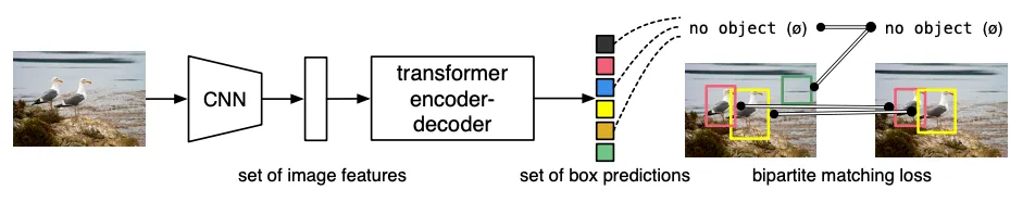
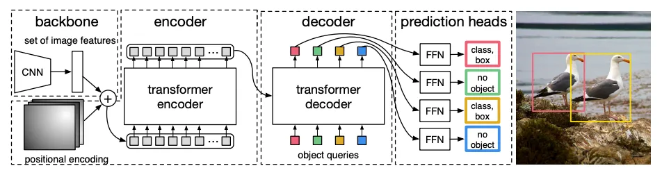
DETR은 object detection을 fixed-size set prediction으로 바꾼다. 전체 구조는 image encoder와 Transformer decoder로 구성된다.

1. CNN backbone이 image feature map을 만든다.
2. Feature map을 token sequence로 펼치고 positional encoding을 더한다.
3. Transformer encoder가 image token을 처리한다.
4. Transformer decoder가 learnable object query와 encoder output을 처리한다.
5. Query마다 class와 bounding box를 출력한다.

Object query는 image patch나 미리 정한 bounding box가 아니다.

$$Q_{\text{obj}} \in \mathbb{R}^{N_q \times d}$$

각 row는 학습 가능한 parameter이며 하나의 output slot 역할을 한다.

각 object query는 특정 클래스와 특정 좌표를 직접 외우는 것이 아니라, 객체 하나를 찾아내기 위한 학습 가능한 detection slot으로 최적화된다.

Decoder 안에서는 query끼리 self-attention하고, encoder image token과 cross-attention한다.

각 query output은 class probability와 normalized bounding box를 만든다.

$$(p_i,b_i) = \operatorname{Head}(z_i)$$

Class에는 실제 object class 외에 no object class가 포함된다. Query 수가 $N_q$이면 최대 $N_q$개의 object를 출력할 수 있다. Image에 object가 더 많으면 전부 표현할 수 없으므로 충분한 query 수를 정해야 한다.

Bipartite matching

Ground-truth object에는 순서가 없으므로 query 1이 특정 object를 맡아야 한다고 미리 정할 수 없다. DETR은 predicted set과 ground-truth set 사이의 minimum-cost bipartite matching을 구한다.

$$\hat{\sigma} = \arg\min_{\sigma} \sum_{j=1}^{N_{\text{gt}}} \mathcal{C} \left( y_j, \hat{y}_{\sigma(j)} \right)$$

Matching cost에는 class error와 box distance, IoU 계열 cost가 들어간다. Matching된 pair에는 class와 box loss를 적용하고, 남은 query는 no object를 예측하도록 학습한다.

$$L_{\text{DETR}} = L_{\text{cls}} + \lambda_1L_1(b,\hat{b}) + \lambda_{\text{IoU}}L_{\text{IoU}}$$

Set-level matching이 duplicate prediction을 직접 억제하므로 기본 DETR은 hand-designed anchor와 NMS 없이 end-to-end로 학습할 수 있다.

Fully supervised DETR의 class head는 training에서 정의한 class만 출력한다. 새로운 class를 zero-shot으로 찾으려면 text embedding 등을 결합한 open-vocabulary extension이 필요하다.

%% title: DETR의 Set Prediction 구조
%% caption: Learnable object query 각각이 하나의 output slot이 되며, image token을 cross-attention한 뒤 class와 box를 예측한다. 학습 시 bipartite matching으로 정답 object와 예측 slot을 연결한다.
flowchart LR
    image["Image"] --> cnn["CNN Backbone"]
    cnn --> tokens["Flattened Image Tokens<br/>+ Position Encoding"]
    tokens --> encoder["Transformer Encoder"]
    queries["Learnable Object Queries<br/>Nq × d"] --> decoder["Transformer Decoder"]
    encoder --> decoder
    decoder --> slots["Nq Query Outputs"]
    slots --> heads["Class Head + Box Head"]
    heads --> set["Predicted Set<br/>{class, box, no-object}"]
    gt["Ground-Truth Object Set"] -.-> match["Bipartite Matching"]
    set -.-> match
    match --> loss["Matched Set Loss"]

Mask R-CNN과 instance segmentation

Mask R-CNN은 Faster R-CNN에 object별 binary mask branch를 추가한다.

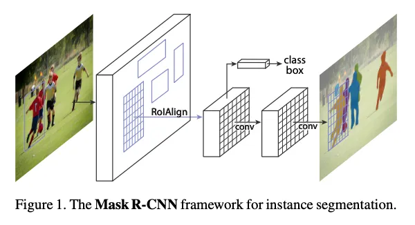
Mask R-CNN의 mask branch는 검출된 bounding box 내부에서 각 pixel이 해당 object에 속하는지 여부를 예측한다. 따라서 semantic segmentation처럼 이미지 전체에 하나의 class map을 만드는 것이 아니라, 각 ROI마다 독립적인 object mask를 생성한다. 같은 class의 object가 여러 개 있어도 ROI가 서로 다르므로 각각 별도의 mask를 얻을 수 있다.

$$\text{ROI feature} \rightarrow \begin{cases} \text{Class head} \\ \text{Box head} \\ \text{Mask head} \end{cases}$$

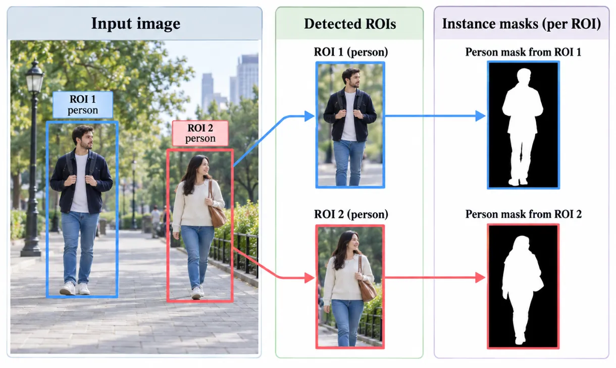
Mask head는 각 ROI 안에서 class별 pixel mask를 예측하는 작은 FCN이다. 전체 loss는 세 task의 합이다.

$$L = L_{\text{cls}} + L_{\text{box}} + L_{\text{mask}}$$

$L_{\text{mask}}$는 해당 object의 binary mask에 대한 pixel-wise binary cross-entropy로 계산할 수 있다.

Mask R-CNN은 ROI pooling의 coordinate quantization(좌표 양자화)을 줄이기 위해 ROIAlign을 사용한다.

정확한 공간 정렬이 필요한 mask prediction에서 작은 위치 오차도 boundary 품질을 떨어뜨리기 때문이다.

ROIAlign은 ROI를 feature map에서 고정된 크기의 특징으로 추출할 때, 좌표를 정수로 반올림하지 않고 실수 좌표를 그대로 사용하는 방법이다.

ROI Pooling은 ROI 경계를 정수 grid에 맞추는 과정에서 좌표 양자화가 발생할 수 있다.

예를 들어 ROI 경계가 $x=12.7$이라면 이를 $x=12$ 또는 $x=13$처럼 정수 좌표로 맞추면서 위치 오차가 생긴다.

ROIAlign은 이런 반올림을 하지 않고, 실수 위치의 특징값을 bilinear interpolation(이중선형 보간)으로 계산한다.

즉 $F(x,y)$가 정수 grid에 없는 위치라면 주변 네 개의 특징값을 가중평균하여 값을 구한다.

이렇게 하면 ROI와 원래 object 위치 사이의 공간 정렬을 더 정확하게 유지할 수 있어, 픽셀 단위 mask prediction에 유리하다.

Model visualization의 목적

Classification accuracy만으로는 model이 올바른 근거를 사용했는지 알 수 없다. 객체 자체가 아니라 배경이나 데이터셋의 우연한 패턴을 보고 정답을 맞힐 수도 있기 때문이다. Model visualization은 prediction에 영향을 준 image 영역과 내부 feature를 확인해 모델의 판단 근거를 살펴보는 데 목적이 있다.

Linear classifier에서는 weight vector를 원래 image shape로 바꾸면 class template처럼 볼 수 있었다. CNN의 첫 convolution filter도 RGB image로 시각화하면 edge, orientation, color contrast 같은 low-level pattern을 확인할 수 있다.

깊은 layer는 channel 수가 많고 feature가 추상적이어서 weight 자체를 그대로 image로 표현하기 어렵다. 이때 input gradient나 activation을 이용해 prediction과 image 위치를 연결한다.

Saliency map(현저성 지도)

Saliency map은 어떤 입력 픽셀이 class score에 영향을 주었는지 보여준다. 예를 들어 의료 영상에서는 종양 유무뿐 아니라 모델이 실제 종양 위치를 근거로 판단했는지도 확인할 수 있다.

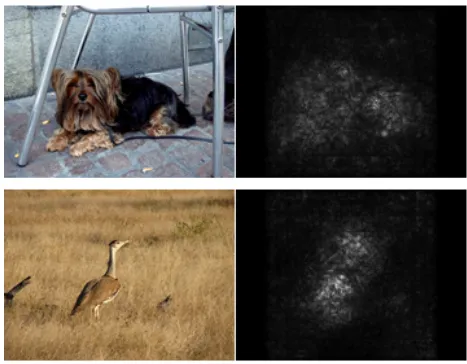
Class $c$의 score를 $s_c(X)$라고 하자. Input pixel을 조금 바꿨을 때 score가 얼마나 변하는지는 input에 대한 gradient로 알 수 있다.

$$G = \frac{\partial s_c}{\partial X}$$

$|G_{i,j,k}|$가 크면 해당 pixel channel의 작은 변화가 class score에 큰 영향을 준다는 뜻이다. RGB channel을 하나의 map으로 줄이려면 channel 방향 absolute maximum 등을 사용할 수 있다.

$$M_{i,j} = \max_k \left| \frac{\partial s_c}{\partial X_{i,j,k}} \right|$$

Saliency map은 별도의 학습 없이 한 번의 backward pass로 계산할 수 있다. 다만 local sensitivity를 보는 방법이므로 gradient noise, activation saturation에 민감하고 object 전체보다 edge처럼 좁은 영역이 강조될 수 있다.

CAM(Class Activation Mapping)

CAM은 마지막 convolution feature map과 class classifier weight를 이용해 class별 spatial heat map을 만든다.

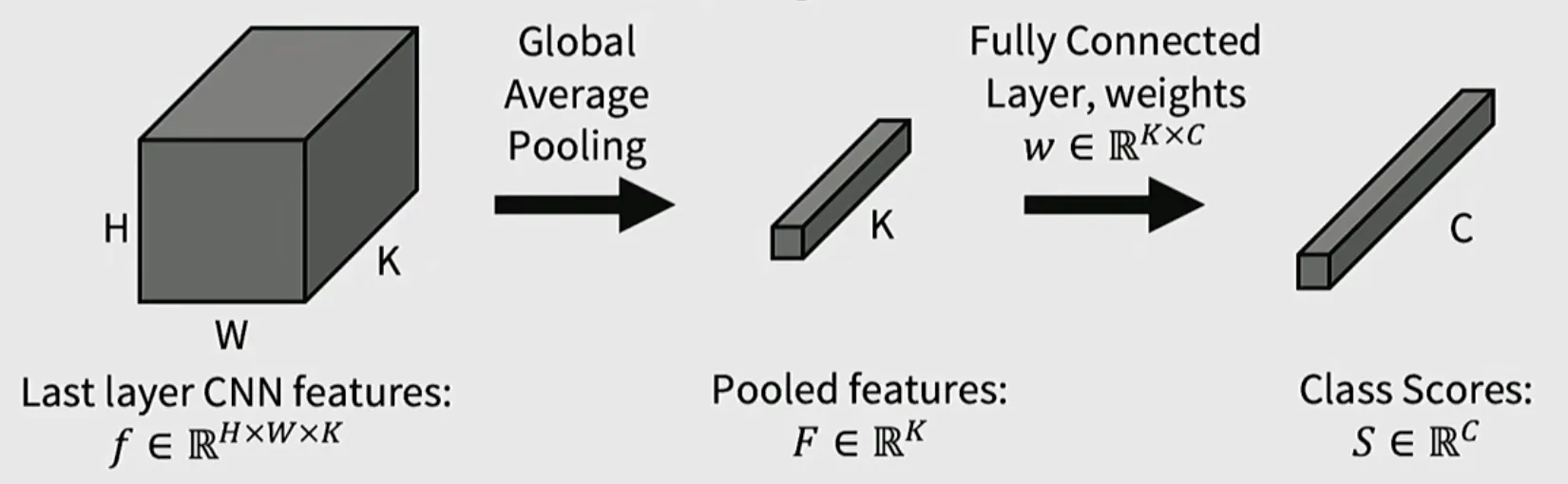
이 절에서 $H$, $W$는 마지막 feature map의 높이와 너비이고, $K$는 channel 수, $C$는 class 수이다.

$$f \in \mathbb{R}^{H \times W \times K}$$

GAP(Global Average Pooling)을 적용하면 channel별 pooled feature $F_k$를 얻는다.

$$F \in \mathbb{R}^{K}$$ $$F_k = \frac{1}{HW} \sum_{h,w}f_{h,w,k}$$

Classifier weight와 class score의 shape는 다음과 같다.

$$w \in \mathbb{R}^{K \times C}, \qquad S \in \mathbb{R}^{C}$$

Class $c$의 score는 pooled feature와 classifier weight $w_{k,c}$의 weighted sum으로 계산한다.

$$\begin{aligned} S_c &= \sum_k w_{k,c}F_k \\ &= \frac{1}{HW} \sum_k w_{k,c} \sum_{h,w}f_{h,w,k} \\ &= \frac{1}{HW} \sum_{h,w} \sum_k w_{k,c}f_{h,w,k} \end{aligned}$$

각 class의 공간 위치별 값을 모은 class activation map의 shape는 다음과 같다.

$$M \in \mathbb{R}^{C \times H \times W}$$

위치 $(h,w)$에서 class $c$에 대한 activation은 다음과 같다.

$$M_{c,h,w} = \sum_k w_{k,c}f_{h,w,k}$$

전체 class score는 이 activation map을 공간 방향으로 평균한 값이다.

$$S_c = \frac{1}{HW} \sum_{h,w}M_{c,h,w}$$

$w_{k,c}$는 feature channel $k$가 class $c$에 얼마나 기여하는지를 나타낸다. Class $c$의 map $M_{c,:,:}$를 input resolution으로 upsampling하면 palace, dome, church처럼 class마다 서로 다른 위치를 강조하는 heat map을 얻는다.

CAM은 마지막 convolution 뒤에 Global Average Pooling과 linear classifier가 바로 이어지는 특정 architecture가 필요하다. 중간에 arbitrary fully connected layer가 있으면 class weight를 feature map에 직접 연결하기 어렵다.

Grad-CAM(Gradient-weighted Class Activation Mapping)

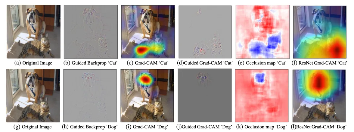
Grad-CAM은 class score의 gradient를 사용해 CAM을 임의의 convolution layer로 일반화한다. 먼저 선택한 layer의 activation을 다음과 같이 둔다.

$$A \in \mathbb{R}^{H \times W \times K}$$

Class score $S_c$를 activation $A$로 미분한 gradient도 같은 shape를 가진다.

$$\frac{\partial S_c}{\partial A} \in \mathbb{R}^{H \times W \times K}$$

이 gradient를 공간 방향으로 Global Average Pooling하면 channel별 weight $\alpha$를 얻는다.

$$\alpha \in \mathbb{R}^{K}$$ $$\alpha_k = \frac{1}{HW} \sum_{h,w} \frac{\partial S_c}{\partial A_{h,w,k}}$$

Class $c$의 Grad-CAM activation map은 다음 shape를 가진다.

$$M^c \in \mathbb{R}^{H \times W}$$

각 위치에서는 activation을 $\alpha_k$로 weighted sum한 뒤 ReLU(Rectified Linear Unit)를 적용한다.

$$M_{h,w}^c = \operatorname{ReLU} \left( \sum_k\alpha_kA_{h,w,k} \right)$$

$\alpha_k$는 $S_c$의 gradient에서 계산되므로 class마다 달라진다. ReLU는 class score를 높이는 positive contribution에 집중한다. Heat map을 input image 크기로 upsampling해 원본 위에 겹치면 model이 해당 class를 판단할 때 사용한 영역을 볼 수 있다.

CAM과 Grad-CAM의 차이는 다음과 같다.

방법	Channel weight	적용 조건
CAM	classifier의 learned weight$w_{k,c}$	GAP 뒤에 linear classifier가 있는 구조
Grad-CAM	gradient average$\alpha_k$	gradient를 계산할 수 있는 임의의 conv layer

Grad-CAM은 더 넓은 architecture에 적용할 수 있지만 heat map resolution은 선택한 feature map resolution에 제한된다.

%% title: Grad-CAM Heat Map 생성 과정
%% caption: 특정 class score를 선택한 convolution feature map까지 역전파하고, channel별 gradient를 가중치로 사용해 spatial activation을 합성한다.
flowchart LR
    image["Input Image"] --> model["CNN Forward"]
    model --> feature["Selected Activations<br/>A ∈ R^(H×W×K)"]
    model --> score["Target Class Score<br/>S_c"]
    score --> backward["Backward to A"]
    backward --> weights["Spatial Mean of Gradients<br/>α_k"]
    feature --> combine["Weighted Sum<br/>Σ_k α_k A[h,w,k]"]
    weights --> combine
    combine --> relu["ReLU + Upsample"]
    relu --> overlay["Heat Map Overlay"]

Transformer attention visualization

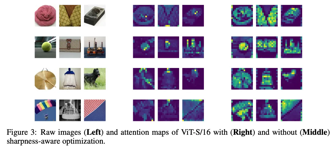
Vision Transformer는 patch token 사이의 attention matrix를 내부에서 직접 계산한다.

$$A^{(h)} = \operatorname{softmax} \left( \frac{Q^{(h)}K^{(h)T}}{\sqrt{d_k}} \right)$$

Class token이 각 patch token에 주는 attention weight를 2차원 patch grid로 되돌리면 어느 image 영역을 참고했는지 시각화할 수 있다. 여러 layer와 head가 있으므로 특정 head 하나를 보거나 head를 평균하고, layer 사이의 attention을 누적하는 방법을 사용할 수 있다.

Attention weight가 높다는 사실만으로 해당 patch가 prediction의 원인이라고 단정할 수는 없다. Residual connection, FFN(Feed-Forward Network), 여러 head와 layer가 함께 output을 만들기 때문이다. Attention map은 유용한 내부 visualization이지만 완전한 explanation은 아니다.

Dense prediction과 visualization의 큰 흐름

각 방법은 image prediction을 spatial location과 연결하는 방식이 다르다.

방법	Spatial output을 얻는 방식	핵심 아이디어
FCN / U-Net	decoder가 pixel score map 생성	encoder의 context와 decoder의 resolution 복원
R-CNN 계열	proposal마다 class와 box 예측	object candidate를 먼저 찾는 two-stage detection
YOLO	dense grid에서 box와 class 동시 예측	한 번의 forward pass로 빠른 detection
DETR	learned query마다 object 하나 예측	attention과 set matching 기반 end-to-end detection
Mask R-CNN	detection ROI마다 binary mask 예측	detection과 segmentation의 결합
Saliency	class score의 input gradient	pixel 변화에 대한 local sensitivity
CAM / Grad-CAM	feature map의 class별 weighted sum	prediction을 convolution 공간에 역으로 연결

Task가 달라도 공통 질문은 같다. Model이 image의 어느 위치에서 어떤 단위의 정보를 만들고, 그 spatial information을 최종 prediction까지 어떻게 보존하는지를 추적해야 한다.