핵심 한 줄 정리

Self-supervised learning(자기지도학습)은 label이 없는 data 자체에서 학습 목표를 만들고, reconstruction이나 contrastive objective를 통해 다양한 downstream task에 재사용할 수 있는 representation을 학습하는 방법이다.

중요 개념 정리

Self-supervised learning이 필요한 이유

Supervised learning은 input과 사람이 만든 label의 쌍을 사용한다. Image classification의 class label도 비용이 들지만, object detection의 bounding box나 semantic segmentation의 pixel label은 훨씬 더 많은 작업을 요구한다. 새로운 domain으로 옮길 때마다 같은 규모의 label을 다시 만드는 것도 어렵다.

반면 image, video, text 같은 raw data는 label보다 훨씬 쉽게 모을 수 있다. Self-supervised learning은 사람이 별도의 정답을 붙이지 않고 data가 이미 가진 구조로 target을 만든다.

예를 들어 image를 회전한 뒤 회전 각도를 맞히게 하면 input을 변형한 기록이 곧 정답이 된다. Image 일부를 가리고 원래 pixel을 복원하게 하면 가리기 전 image가 target이 된다. 같은 image에서 만든 두 augmentation을 서로 가깝게 만들 때는 두 view가 같은 source에서 왔다는 사실이 supervision이 된다.

따라서 self-supervised learning에서 self는 model이 스스로 의식을 가지고 학습한다는 뜻이 아니라, supervision을 data 자체로부터 구성한다는 뜻이다.

Pretraining과 downstream task

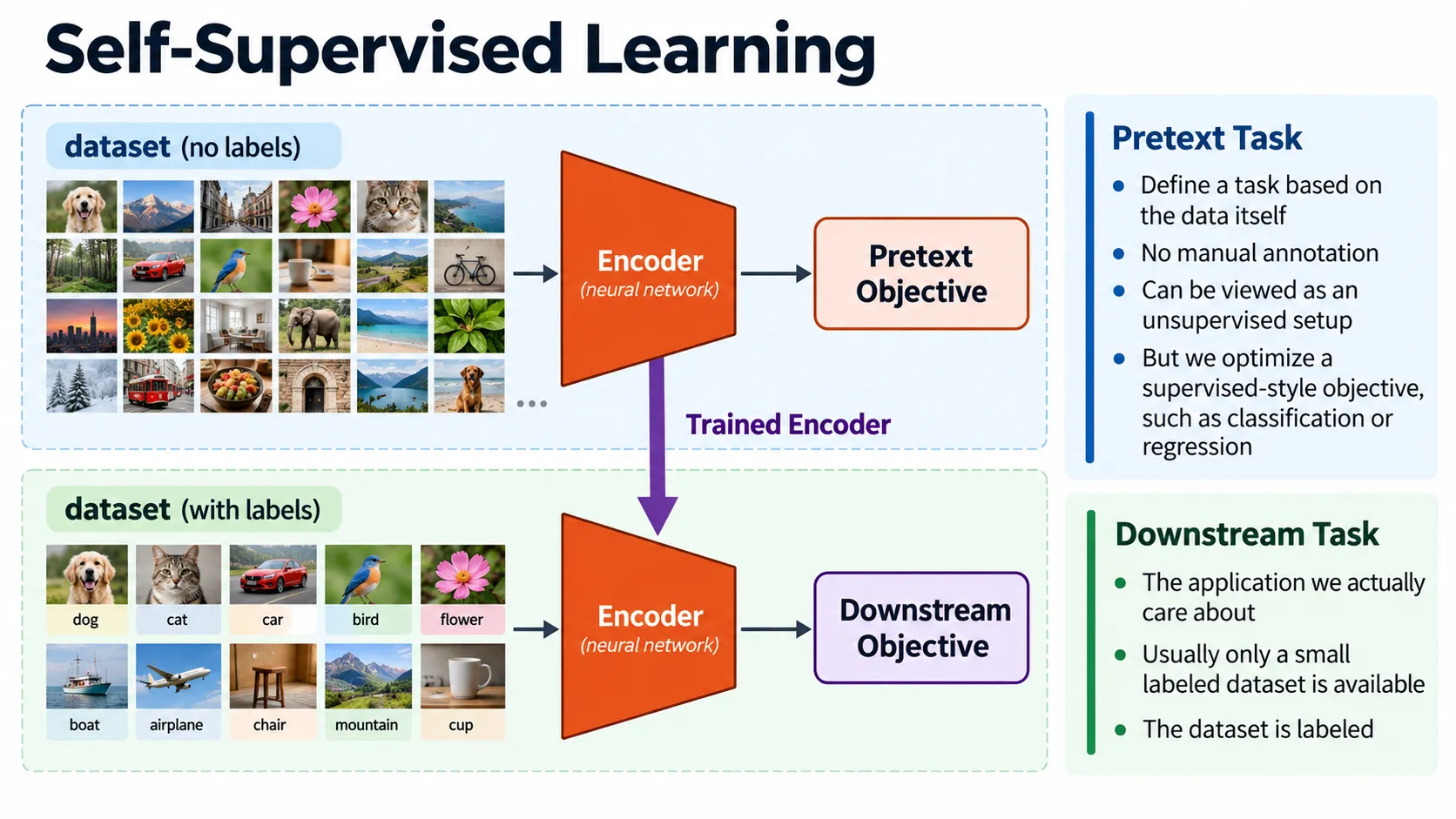
Pretext task는 사람이 label을 붙이는 대신 data 자체에서 target을 만들어 encoder를 학습시키는 사전 학습용 task이다. 회전 각도 예측, 가려진 영역 복원 등이 이에 해당하며, task 자체를 잘 푸는 것보다 downstream task에 재사용할 representation을 얻는 것이 목적이다.

Self-supervised learning은 보통 representation을 먼저 학습하고, 이후 label이 있는 task에 옮겨 쓰는 두 단계로 구성된다.

1. Label이 없는 대규모 data로 encoder를 pretrain한다.
2. Pretext task에만 필요했던 prediction head나 decoder를 제거한다.
3. Encoder가 만든 feature를 classification, detection, segmentation 같은 downstream task에 사용한다.

Input $x$를 encoder $f_\theta$에 통과시킨 representation을 다음과 같이 나타낼 수 있다.

$$h = f_\theta(x)$$

$h$는 representation, feature, embedding, latent vector 등으로 불린다. 표현은 조금씩 다르지만, raw input을 downstream task에서 사용하기 좋은 형태로 변환한 내부 표현이라는 공통점이 있다.

Pretext head $g_\phi$까지 포함한 pretraining objective는 일반적으로 다음과 같이 쓸 수 있다.

$$\theta^*,\phi^* = \arg\min_{\theta,\phi} \mathbb{E}_{x \sim \mathcal{D}} \left[ \mathcal{L}_{\text{pretext}} \left(g_\phi(f_\theta(x)),t(x)\right) \right]$$

$t(x)$는 raw data $x$에서 자동으로 만든 target이다. Pretraining이 끝나면 $g_\phi$보다 encoder $f_{\theta^*}$가 핵심 결과물이다.

좋은 pretext task는 그 task만 푸는 shortcut보다 object의 shape, texture, part, context, correspondence 같은 재사용 가능한 정보를 학습하게 해야 한다. Pretext loss가 낮다는 사실만으로 representation이 좋다고 결론 내릴 수 없는 이유이다.

%% title: Self-Supervised Pretraining에서 Downstream Transfer까지
%% caption: Label 없는 data와 자동 생성 target으로 encoder를 pretrain한 뒤, pretext 전용 head는 버리고 encoder representation을 새 task에 재사용한다.
flowchart LR
    raw["Unlabeled Raw Data"] --> target["Automatic Target t(x)<br/>mask · augmentation · context"]
    raw --> encoder["Encoder fθ"]
    encoder --> prehead["Pretext Head gφ"]
    target --> preloss["Self-Supervised Loss"]
    prehead --> preloss
    preloss -. "pretrain" .-> encoder
    encoder --> frozen["Frozen Encoder<br/>Linear Probe"]
    encoder --> finetune["Encoder + Task Head<br/>Fine-tuning"]
    frozen --> downstream["Classification · Detection · Segmentation"]
    finetune --> downstream

Representation을 평가하는 방법

Self-supervised model은 pretext task의 정확도보다 downstream task에서 얼마나 잘 전이되는지로 평가해야 한다.

Linear probing

Pretrained encoder의 parameter를 고정하고 그 위에 linear classifier만 학습한다.

$$h_i = f_{\theta^*}(x_i)$$ $$\hat{y}_i = Wh_i+b$$

Encoder를 바꾸지 않으므로 representation 안에 class를 선형적으로 구분할 정보가 이미 들어 있는지를 확인할 수 있다. Encoder의 도움을 받아 전체 model이 새 task에 적응하는 능력보다, feature 자체의 품질을 비교하는 데 적합하다.

Fine-tuning

Pretrained encoder와 새 task의 head를 함께 학습한다. Linear probing보다 model의 적응 범위가 넓어 일반적으로 성능이 높지만, optimization 설정과 label 수의 영향을 더 크게 받는다.

그 밖의 평가

• Frozen feature에 k-nearest neighbor를 적용할 수 있다.
• Object detection과 semantic segmentation처럼 classification과 다른 task로 transfer할 수 있다.
• Label이 적은 조건에서 sample efficiency를 비교할 수 있다.
• Corruption, distribution shift, adversarial perturbation에 대한 robustness를 볼 수 있다.
• t-SNE나 nearest-neighbor retrieval로 embedding을 시각화할 수 있지만, 이는 정성적인 근거이므로 downstream metric을 대신하지 못한다.

Rotation prediction

Rotation prediction은 image를 $0^\circ$, $90^\circ$, $180^\circ$, $270^\circ$ 중 하나로 회전하고, 어느 각도인지 맞히는 4-class classification task이다.

$$r \in \{0,1,2,3\}$$ $$x^{(r)} = \operatorname{Rotate}(x,90r^\circ)$$ $$\mathcal{L}_{\text{rot}} = -\log p_\theta \left(r\mid x^{(r)}\right)$$

정답은 rotation transform을 적용할 때 자동으로 얻는다. Model이 angle을 맞히려면 object의 정상적인 방향, part의 배치, scene의 위아래와 같은 visual structure를 알아야 한다는 가정이다.

CIFAR-10 classification에 transfer하면 rotation pretraining을 사용한 model은 random initialization보다 높은 accuracy에서 시작한다. 단순한 supervised task를 충분히 오래 학습하면 차이가 줄어들 수 있지만, label이 적거나 downstream task가 복잡할수록 좋은 initialization의 가치가 커진다.

아래 결과는 ImageNet의 label 없이 rotation prediction으로 AlexNet을 pretrain한 뒤 PASCAL VOC(PASCAL Visual Object Classes)의 classification, detection, segmentation에 fine-tuning한 결과이다.

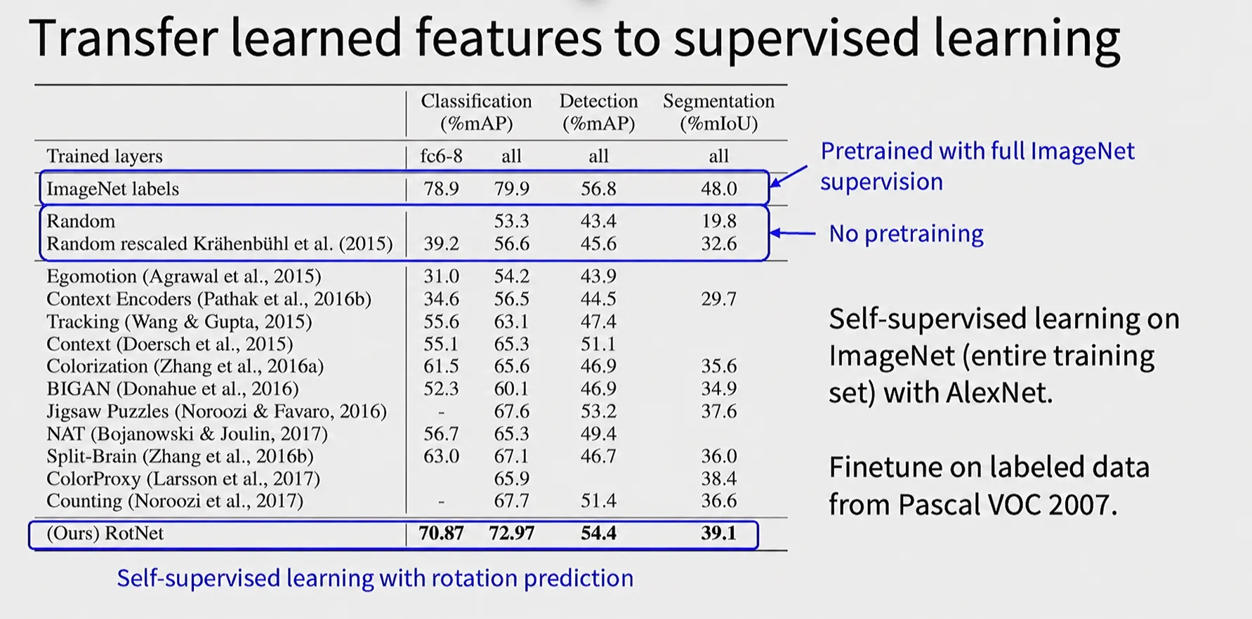
RotNet은 세 task 모두에서 random initialization보다 높은 transfer 성능을 보였다. ImageNet supervised pretraining에는 미치지 못했지만, class label 없이도 downstream task에 유용한 visual representation을 학습할 수 있음을 보여준다.

Transfer 성능: 한 작업에서 학습한 feature가 다른 작업에서도 얼마나 유용하게 활용되는지를 나타내는 성능

다만 rotation prediction에는 shortcut이 생길 수 있다. Camera artifact, border pattern, 특정 background처럼 angle과 우연히 연관된 단서를 이용하면 object를 이해하지 않고도 task를 풀 수 있다. Pretext task를 설계할 때 target만 자동 생성하면 되는 것이 아니라 shortcut도 함께 점검해야 한다.

Relative patch position

Relative patch position task는 image에서 두 patch를 뽑고, 두 번째 patch가 첫 번째 patch의 어느 방향에 있는지 예측한다. 중심 patch 주변을 $3 \times 3$ grid로 보면 중심을 제외한 8개 위치가 class가 된다.

$$y \in \{\text{top-left},\text{top},\ldots,\text{bottom-right}\}$$

두 patch 사이의 상대 위치를 맞히려면 object part와 scene layout의 관계를 학습해야 한다. 예를 들어 얼굴의 눈 위에는 이마가 있고, 자동차 wheel은 body 아래에 있다는 식의 spatial regularity가 feature에 반영될 수 있다.

하지만 chromatic aberration이나 patch boundary처럼 camera와 sampling 과정에서 생긴 단서를 이용할 수도 있다. 그래서 patch 사이에 gap을 두거나 color channel을 변형해 shortcut을 줄이는 방법이 함께 사용된다.

Jigsaw puzzle

Jigsaw task는 image를 $3 \times 3$ patch로 나눈 뒤 순서를 섞고, 원래 배치를 복원하게 한다. Patch 9개의 모든 permutation은 다음과 같이 매우 많다.

$$9! = 362{,}880$$

모든 permutation을 class로 사용하면 classification problem이 지나치게 커진다. 실제 예에서는 서로 충분히 다른 64개 permutation을 골라 64-class classification으로 학습한다.

서로 비슷한 permutation만 선택하면 class 사이 차이가 작아지고, 반대로 잘 분리된 permutation을 사용하면 각 class가 다른 global arrangement를 나타낸다. 모델은 local texture만 보는 대신 part 사이의 배치와 object-level structure를 사용해야 한다.

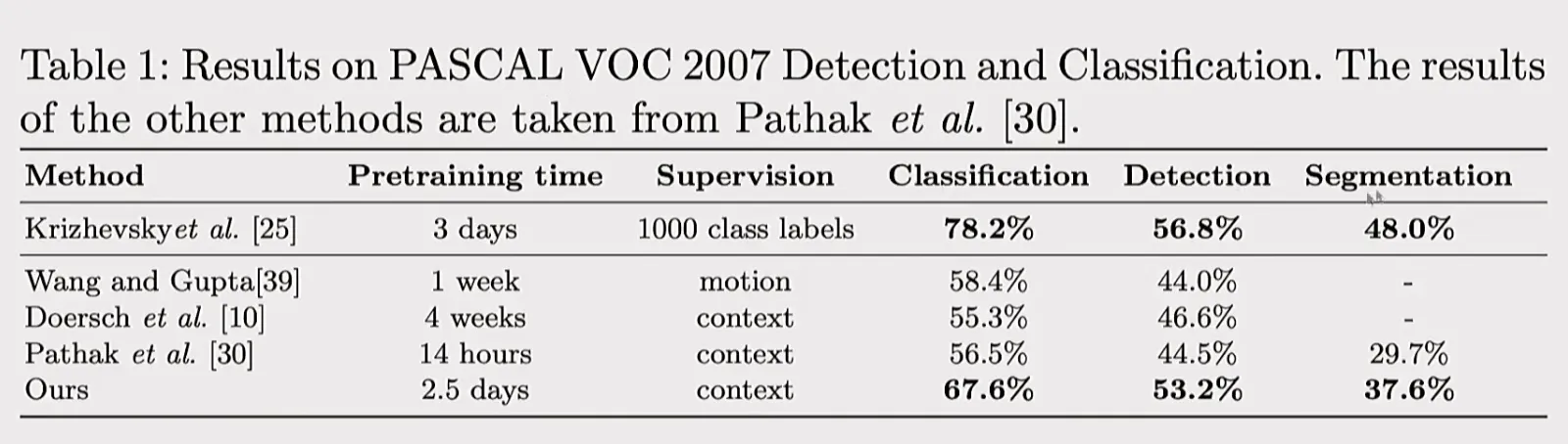
Jigsaw 방식으로 사전 학습한 모델은 PASCAL VOC 2007의 classification에서 67.6%, object detection에서 53.2%, semantic segmentation에서 37.6%를 기록하였다. ImageNet label로 사전 학습한 모델에는 미치지 못하지만, 기존 self-supervised learning 방식보다 전반적으로 높은 transfer 성능을 보였다. 이는 조각의 상대적 배치를 맞히는 pretext task가 물체의 형태와 공간적 맥락을 담은 representation을 학습하는 데 도움이 된다는 것을 보여준다.

Relative position과 jigsaw는 spatial context를 학습한다는 장점이 있지만, patch의 low-level boundary나 고정된 permutation set에 과도하게 맞춰질 수 있다.

Context encoder와 Predict Missing Pixels (inpainting)

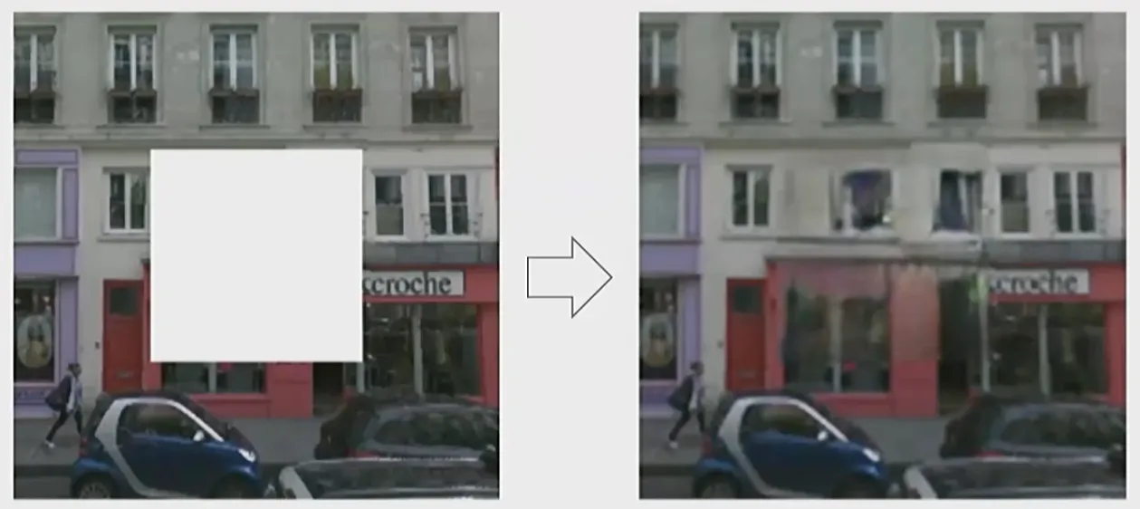
Inpainting은 image 일부를 mask로 가린 뒤 missing region의 pixel을 복원하는 task이다. Encoder는 보이는 context를 representation으로 만들고, decoder는 그 representation으로 가려진 영역을 예측한다.

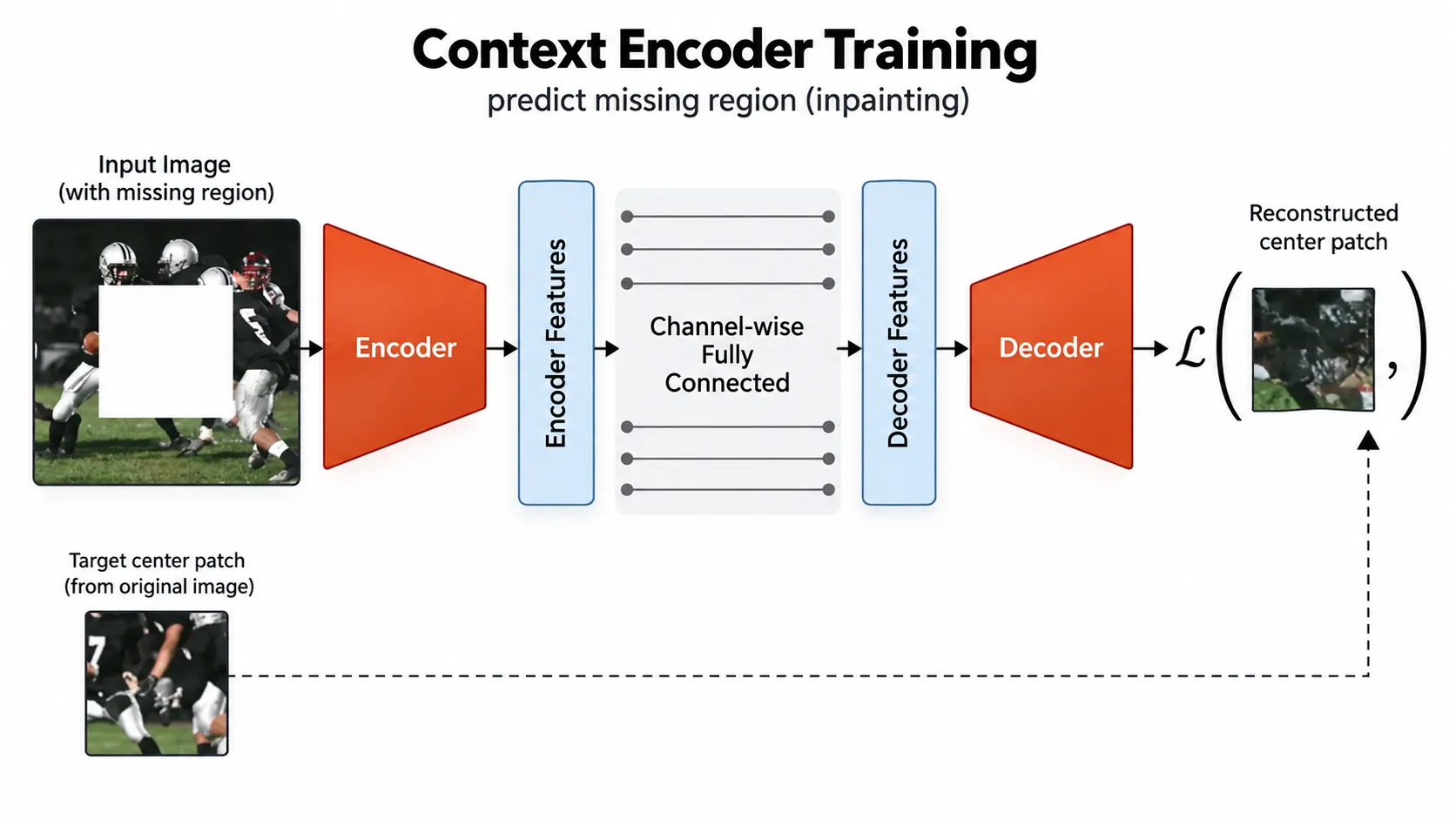
초기 context encoder는 reconstruction loss와 adversarial loss를 함께 사용한다. Original image를 $x$, 가려진 pixel에서 1이고 나머지에서 0인 mask를 $M$이라고 하면 복원 결과는 다음과 같다.

$$\hat{x} = F_\theta\left((1-M)\odot x\right)$$

강의 슬라이드의 reconstruction loss는 가려진 영역의 squared error를 모두 더하는 합계 형태이다.

$$\mathcal{L}_{\text{recon}}^{\text{sum}}(x) = \left\lVert M\odot(x-\hat{x}) \right\rVert_2^2$$

기존 수식처럼 가려진 pixel 수 $\lVert M\rVert_1$로 나누면 masked pixel당 평균을 계산하는 형태가 된다.

$$\mathcal{L}_{\text{recon}}^{\text{mean}}(x) = \frac{1}{\lVert M\rVert_1} \mathcal{L}_{\text{recon}}^{\text{sum}}(x) = \frac{1}{\lVert M\rVert_1} \left\lVert M\odot(x-\hat{x}) \right\rVert_2^2$$

슬라이드에서는 $\mathcal{L}_{\text{recon}}(x)=\mathcal{L}_{\text{recon}}^{\text{sum}}(x)$으로 두고 전체 objective를 다음과 같이 나타낸다.

$$\mathcal{L}(x) = \mathcal{L}_{\text{recon}}(x) + \mathcal{L}_{\text{adv}}(x)$$ $$\mathcal{L}_{\text{adv}} = \max_D \mathbb{E}_{x} \left[ \log D(x) + \log \left( 1-D\left(F_\theta\left((1-M)\odot x\right)\right) \right) \right]$$

$x$는 original image이고, $M$은 가린 pixel에서 1, 나머지에서 0인 mask이다. 따라서 $(1-M)\odot x$는 일부 영역이 가려진 input이며, $F_\theta$는 이를 바탕으로 전체 image $\hat{x}$를 복원한다. $\odot$는 element-wise multiplication이다. Reconstruction loss는 $M$을 곱해 가려진 영역에서만 원본과 복원 결과의 차이를 계산한다. 합계 형태와 평균 형태는 mask 크기가 고정되어 있고 reconstruction loss만 고려할 때 상수 배 차이이므로 같은 최적해를 갖는다. Mask 크기가 달라지면 평균 형태가 큰 mask에 과도한 가중치가 실리는 것을 막는다. 다만 adversarial loss와 함께 사용할 때는 정규화 여부에 따라 두 loss의 상대적인 크기가 달라지므로 loss weight도 함께 조정해야 한다. Adversarial loss에서 discriminator $D$는 원본 image와 복원 image를 구분하도록 학습되고, $F_\theta$는 복원 결과가 실제 image처럼 보이도록 학습된다.

Pixel-wise L2 loss에는 한계가 있다. 가려진 영역에 여러 개의 그럴듯한 정답이 있을 때 L2 objective는 그 후보들의 평균에 가까운 값을 선호한다. 서로 다른 texture와 edge를 평균내면 reconstruction이 흐릿해진다.

Adversarial loss는 이러한 흐릿한 평균 대신 실제 image patch처럼 자연스러운 결과를 만들도록 보완한다. 다만 inpainting을 representation learning에 사용할 때 downstream에 가져가는 것은 decoder가 아니라 encoder이다.

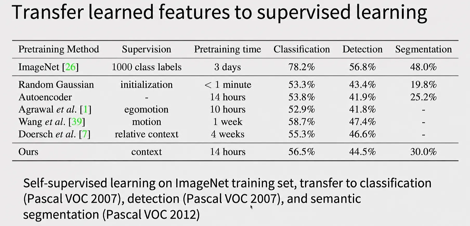
Context Encoder로 사전 학습한 encoder는 PASCAL VOC의 classification에서 56.5%, object detection에서 44.5%, semantic segmentation에서 30.0%를 기록하였다. ImageNet label을 사용한 supervised pretraining에는 미치지 못하지만, random initialization보다 특히 semantic segmentation에서 높은 성능을 보여 inpainting으로 학습한 representation이 downstream task에도 전이됨을 보여준다.

Colorization과 split-brain autoencoder

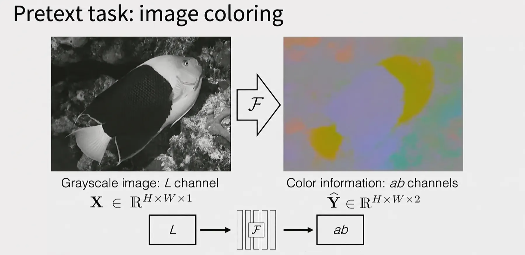
LAB color space는 밝기를 나타내는 $L$ channel과 색 정보를 나타내는 $a,b$ channel로 나뉜다. Colorization은 grayscale에 해당하는 $L$을 input으로 받고 $ab$를 예측한다.

$$L \longrightarrow (a,b)$$

Object의 그럴듯한 색을 복원하려면 sky, grass, skin, vehicle처럼 semantic category를 어느 정도 구분해야 한다. 따라서 colorization을 풀기 위해 학습한 encoder feature를 다른 vision task로 transfer할 수 있다.

단순한 L2 regression은 한 위치에 가능한 여러 색을 평균내 회색이나 탁한 색을 만들 수 있다. 색 공간을 bin으로 나누고 각 pixel의 color distribution을 classification으로 예측하면 multimodal uncertainty를 더 잘 표현할 수 있다.

Split-brain autoencoder는 channel을 양방향으로 예측한다.

$$f_1:L\rightarrow(a,b)$$ $$f_2:(a,b)\rightarrow L$$

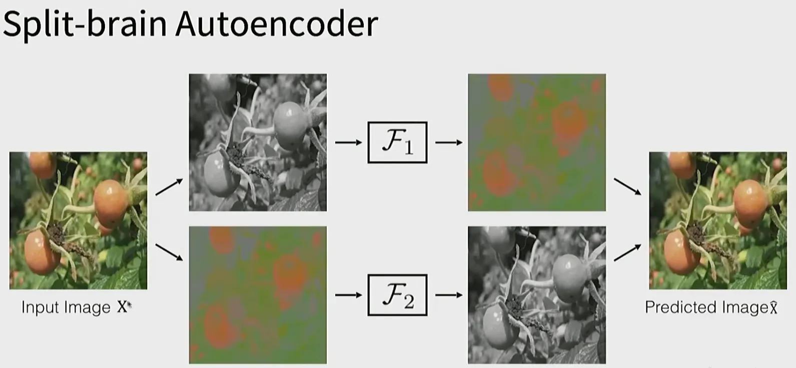
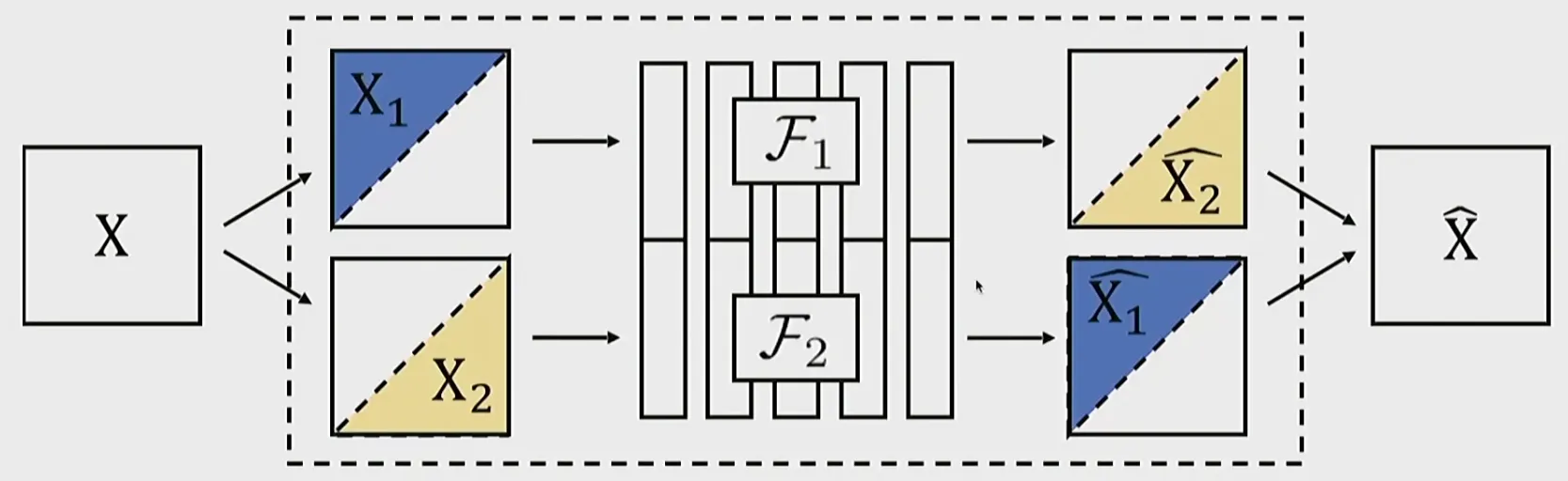
두 network에서 얻은 feature를 concatenate하면 shape와 texture에 가까운 luminance 정보, color에 가까운 chrominance 정보를 함께 담을 수 있다.

이 생각은 LAB에만 한정되지 않는다. RGB와 depth가 함께 있는 data라면 RGB로 depth를 예측하고 depth로 RGB를 예측할 수 있다. 서로 다른 channel이나 modality가 공유하는 structure를 맞히는 것이 supervision이 된다.

Video color propagation으로 correspondence 학습하기

가설: Video frame을 colorize하는 방법을 학습하면 별도의 tracking label 없이도 region이나 object를 추적하는 feature를 학습할 수 있다.

Video의 인접 frame은 장면과 object를 공유하지만 위치가 조금씩 바뀐다. Reference frame에는 color가 있고 target frame은 grayscale이라고 하자. Target frame의 각 pixel이 reference frame의 어느 pixel과 대응하는지 찾은 뒤 그 color를 가져오면 target frame을 colorize할 수 있다.

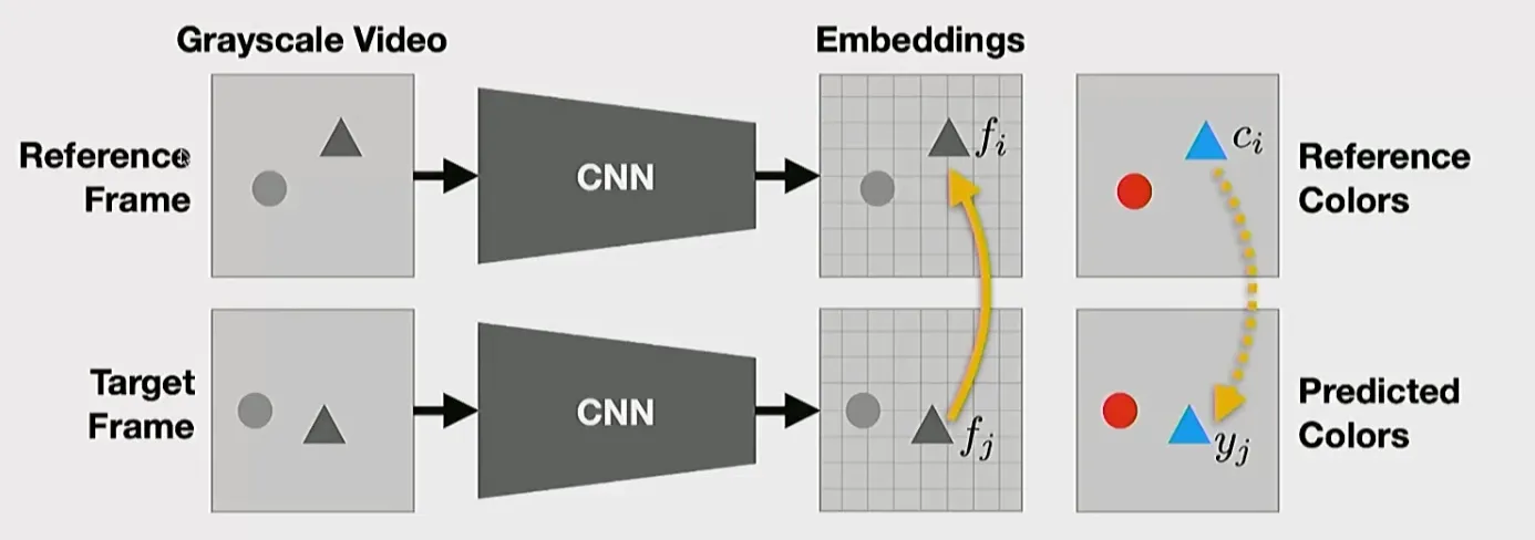
그림의 두 grayscale frame은 밝기와 형상 정보를, 오른쪽의 두 color map은 색 정보를 나타낸다.

• Reference Frame은 대응 관계의 기준이 되는 이전 시점의 frame이다.
• Input Frame은 color를 예측할 다음 시점의 frame이며, 아래 수식에서는 target frame이라고 부른다.
• Reference Colors는 reference frame의 실제 색으로, LAB color space에서는 주로 $a,b$ channel에 해당한다.
• Target Colors는 reference의 색을 input frame의 대응 위치로 옮겨 예측한 결과이다.

예를 들어 reference frame의 왼쪽에 있던 파란 소매가 다음 frame에서 오른쪽으로 이동했다면, model은 두 frame의 feature를 비교해 같은 소매의 새 위치를 찾는다. 그런 다음 reference colors의 파란색을 target의 대응 위치로 전달한다. 즉 reference frame에서 같은 대상을 찾고, 그 대상의 reference color를 input frame의 대응 위치에 옮겨 target color를 만든다.

Reference pixel $i$의 feature를 $f_i^r$, target pixel $j$의 feature를 $f_j^t$라고 하자. Target pixel $j$와 각 reference pixel $i$의 dot-product similarity를 reference frame의 모든 위치에 대해 softmax하면 attention weight는 다음과 같다.

$$A_{ij} = \frac{ \exp\left((f_i^r)^\top f_j^t\right) }{ \sum_k \exp\left((f_k^r)^\top f_j^t\right) }$$

따라서 고정된 target pixel $j$에 대해 $\sum_i A_{ij}=1$이다. Reference pixel $i$의 color $c_i$를 이 weight로 합하면 target pixel $j$의 predicted color $y_j$를 얻는다.

$$y_j = \sum_i A_{ij}c_i$$

예측한 color $y_j$와 target frame의 실제 color $c_j$ 사이의 loss를 모든 target pixel에 대해 합하고, 이를 최소화하도록 feature extractor의 parameter $\theta$를 학습한다.

$$\min_{\theta} \sum_j \mathcal{L}(y_j,c_j)$$

여기서 예측식의 $c_i$는 reference pixel $i$의 color이고, loss의 $c_j$는 target pixel $j$의 ground-truth color이다.

Color propagation만 학습했지만 feature는 frame 사이의 correspondence를 표현하게 된다. 이 correspondence는 object tracking, keypoint matching, segmentation mask propagation 같은 task에도 사용할 수 있다.

학습에는 원래 color video를 사용하므로 실제 target colors를 정답으로 알고 있다. 다만 model input에서는 target의 색을 숨기고 reference colors만으로 이를 예측하게 한다. 따라서 별도의 사람이 만든 label 없이도 frame 사이의 correspondence가 supervision이 된다.

Video에서는 시간적으로 가까운 frame이 비슷하다는 자연스러운 supervision을 얻을 수 있다. Image의 augmentation보다 실제 object motion과 viewpoint 변화가 포함된 positive relation을 제공한다는 장점이 있다.

Downstream task로 feature 평가하기

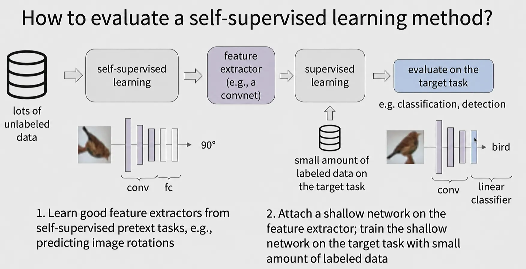
앞에서 살펴본 pretext task가 좋은 feature extractor를 만들었는지는 target task로 옮겨 확인한다. 강의에서 다시 제시한 평가 절차는 다음과 같다.

1. Label이 없는 대규모 data와 self-supervised pretext task로 feature extractor를 학습한다.
2. 학습한 feature extractor를 고정하고 그 위에 linear classifier 같은 shallow network를 붙인다.
3. Target task의 적은 labeled data로 shallow network를 supervised learning한다.
4. Classification이나 detection 같은 target task의 성능을 측정한다.

이 평가는 encoder 자체를 다시 크게 학습시키는 것이 아니라, 이미 학습된 feature가 간단한 classifier만으로 유용하게 분리되는지를 보는 linear evaluation protocol이다. Rotation prediction이나 color propagation의 pretext 성능이 높더라도 downstream 성능이 낮다면 좋은 representation이라고 보기 어렵다.

Encoder와 decoder는 대칭일 필요가 없다

Encoder와 decoder가 하나의 큰 network인지, 서로 분리된 network인지는 pretext task에 따라 달라진다. Rotation prediction에서는 CNN encoder 뒤의 FC classifier까지 하나의 network로 보고 함께 학습한 다음, downstream task에서는 이 classifier를 새로운 task head로 교체할 수 있다. 반면 image autoencoding에서는 encoder와 decoder를 서로 다른 network module로 구성하고 reconstruction loss로 end-to-end 학습하기도 한다.

여기서 대칭적인 autoencoder란 decoder가 encoder의 layer 구성을 거꾸로 펼친 mirror 형태인 구조를 뜻한다.

Encoder: 784 → 512 → 256 → 128
Decoder: 128 → 256 → 512 → 784

하지만 encoder와 decoder가 반드시 이런 대칭 구조일 필요는 없다. MAE는 visible patch만 처리하는 큰 ViT encoder와 pixel reconstruction을 담당하는 훨씬 작은 Transformer decoder를 사용한다. 두 module은 크기와 깊이뿐 아니라 세부 architecture도 다르게 설계할 수 있으며, 중요한 것은 서로 같은 모양인지가 아니라 pretext objective를 end-to-end로 학습할 수 있는지이다.

수작업 pretext task의 한계

Rotation, jigsaw, inpainting, colorization은 label 없이 representation을 학습할 수 있음을 보여주었지만 몇 가지 공통적인 한계가 있다.

• 어떤 transformation과 target이 좋은지는 사람이 직접 설계해야 한다.
• Model이 semantic structure보다 task-specific shortcut을 찾을 수 있다.
• Pretext task를 어렵게 만든다고 downstream representation이 반드시 좋아지지는 않는다.
• Task마다 별도의 head나 decoder가 필요하다.
• Pixel reconstruction은 perceptual similarity와 정확히 일치하지 않는다.
• Invariance를 잘못 정하면 downstream에 필요한 정보까지 제거할 수 있다.

이후 방법들은 보다 단순하고 scale하기 쉬운 objective를 사용한다. Masked Autoencoder는 image 일부를 크게 가리고 복원하며, contrastive learning은 같은 source의 여러 view가 같은 representation을 갖게 한다.

Masked Autoencoder

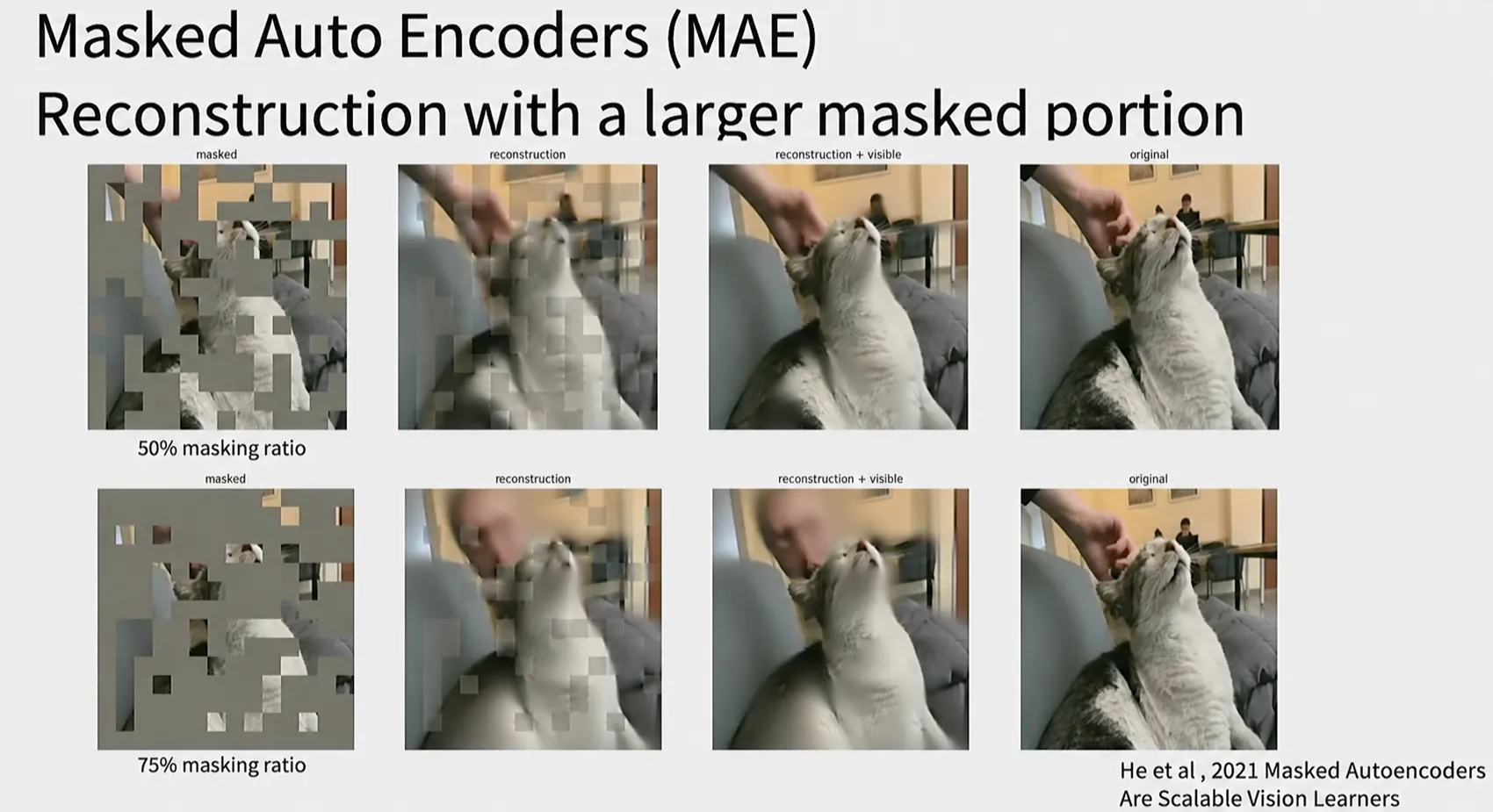
Masked Autoencoder, MAE는 image를 patch로 나누고 대부분의 patch를 가린 뒤 missing patch의 pixel을 복원한다. Rotation, jigsaw, colorization처럼 서로 다른 transformation과 prediction target을 task마다 설계하는 초기 방법과 달리, 원본 pixel 복원이라는 단순하고 범용적인 objective를 사용한다.

기존 context encoder가 주로 하나의 큰 영역을 가리고 복원했다면, MAE는 image 전반의 patch를 무작위로 높은 비율까지 가린다. 매번 다른 mask를 만들 수 있어 같은 image에서도 다양한 학습 sample을 얻고, 주변 pixel만 복사하는 쉬운 해결을 어렵게 만들어 넓은 context와 object structure를 학습하게 한다. 또한 큰 encoder는 visible patch만 처리하고 작은 decoder가 복원을 담당하므로 대규모 ViT pretraining으로 확장하기에도 효율적이다.

Architecture는 큰 ViT encoder와 작은 Transformer decoder의 비대칭 구조이다.

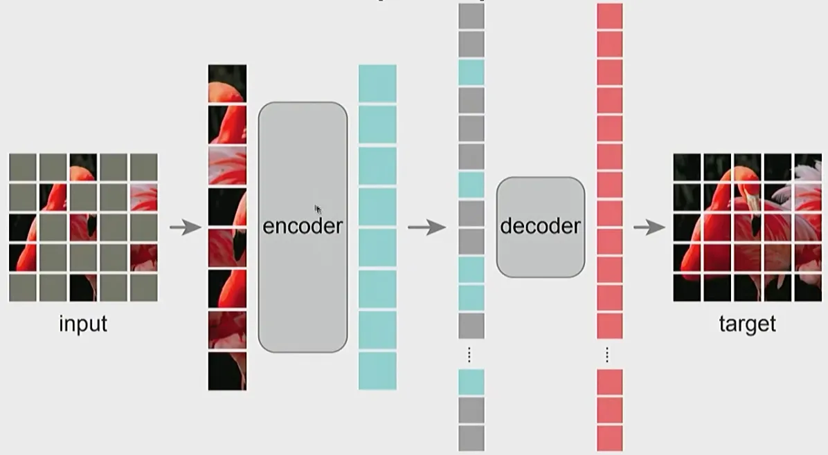
Image를 $N$개의 patch로 나누고 mask index 집합을 $\mathcal{M}$, visible index 집합을 $\mathcal{V}$라고 하자.

$$\mathcal{V} \cup \mathcal{M} = \{1,2,\ldots,N\}$$ $$\mathcal{V} \cap \mathcal{M} = \varnothing$$

Mask ratio가 $75\%$이면 encoder가 보는 patch 수는 전체의 $25\%$이다.

$$|\mathcal{V}| = 0.25N$$

Training 과정은 다음과 같다.

1. Image를 patch로 나누고 각 patch를 vector로 펼친다.
2. Patch의 $75\%$를 random하게 mask한다.
3. Visible patch만 linear projection하고 positional embedding을 더해 ViT encoder에 넣는다.
4. Encoder output에 missing 위치를 나타내는 learnable mask token을 추가한다.
5. 모든 token을 원래 위치 순서로 정렬하고 decoder positional embedding을 더한다.
6. 작은 Transformer decoder가 각 missing patch의 pixel을 예측한다.
7. Loss는 masked patch에 대해서만 계산한다.

Encoder는 mask token을 처리하지 않는다. 전체 token은 lightweight decoder에서 처음 합쳐진다. 이는 BERT처럼 encoder가 visible token과 mask token을 모두 처리하는 방식과 다른 부분이다.

%% title: Masked Autoencoder의 비대칭 구조
%% caption: 큰 encoder는 visible patch 25%만 처리하고, 작은 decoder가 mask token을 포함한 전체 patch 순서를 복원한다. Loss는 masked patch에만 적용한다.
flowchart LR
    image["Image"] --> patches["Patchify<br/>N patches"]
    patches --> mask["Random Mask 75%"]
    mask --> visible["Visible Patches 25%"]
    visible --> encoder["Large ViT Encoder"]
    encoder --> encoded["Visible Representations"]
    masktoken["Learnable Mask Tokens"] --> restore["Restore Original Positions"]
    encoded --> restore
    restore --> decoder["Lightweight Decoder"]
    decoder --> prediction["Predicted Patch Pixels"]
    original["Original Masked Patches"] --> loss["Masked-Only MSE"]
    prediction --> loss

MAE reconstruction objective

Patch $i$의 original pixel vector를 $x_i$, decoder prediction을 $\hat{x}_i$라고 하면 MAE loss는 masked patch에 대한 mean squared error이다.

$$\mathcal{L}_{\text{MAE}} = \frac{1}{|\mathcal{M}|} \sum_{i\in\mathcal{M}} \left\lVert x_i-\hat{x}_i \right\rVert_2^2$$

각 patch를 평균과 표준편차로 normalize한 pixel을 target으로 사용할 수도 있다. 이 경우 local contrast와 texture 차이를 더 균형 있게 다룰 수 있다.

Visible patch의 reconstruction까지 loss에 포함하면 이미 input으로 주어진 pixel을 복사하는 쉬운 항이 loss를 지배할 수 있다. Masked patch에만 loss를 적용해야 context에서 missing content를 추론하는 능력을 직접 학습한다.

Mask ratio가 높은 이유

Image에는 인접 pixel과 patch 사이 redundancy가 크다. Mask ratio가 낮으면 주변 texture를 복사하는 것만으로 reconstruction을 쉽게 풀 수 있고, global semantic structure를 배울 필요가 줄어든다. MAE는 $75\%$라는 높은 mask ratio로 이 shortcut을 어렵게 만든다.

높은 mask ratio는 compute 측면에서도 중요하다. Self-attention의 주요 비용은 token 수 $N$에 대해 대략 $O(N^2)$이다. Encoder에 전체의 $25\%$만 넣으면 attention matrix의 크기는 단순 계산으로 다음 비율까지 줄어든다.

$$\left(0.25N\right)^2 = 0.0625N^2$$

즉 attention 부분만 보면 전체 token을 처리할 때의 약 $6.25\%$이다. 실제 전체 runtime은 projection, MLP, decoder 등의 비용도 있어 정확히 16배 빨라지는 것은 아니지만, 큰 encoder의 pretraining 비용을 크게 줄일 수 있다.

Random mask는 block mask나 규칙적인 grid mask보다 다양한 missing pattern을 만든다. 같은 image에서도 매번 다른 visible subset이 생기므로 일종의 data variation 역할도 한다. 제시된 ablation에서는 random $75\%$ mask가 좋은 transfer 결과를 보였다.

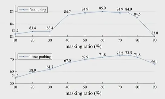
이 실험에서는 fine-tuning 성능이 약 $60\%$ masking에서, linear probing 성능은 약 $75\%$ masking에서 가장 높았다. 따라서 $75\%$가 모든 평가 방식에서 최적이라는 뜻은 아니다.

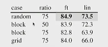
Mask sampling 방식의 비교에서는 $75\%$ random mask가 같은 비율의 block·grid mask보다 높은 성능을 보였다. 표의 block $50\%$ 행은 masking ratio도 다르므로 별도 조건으로 읽어야 한다.

Encoder와 decoder를 비대칭으로 만드는 이유

MAE에서 최종적으로 downstream task에 사용하는 부분은 encoder이다. Decoder는 pretraining target을 복원하기 위한 보조 구조이며 transfer 단계에서는 제거된다.

따라서 다음과 같이 자원을 배분한다.

• Encoder는 큰 capacity를 갖고 transferable representation을 학습한다.
• Decoder는 encoder output을 pixel로 바꾸는 데 필요한 최소한의 depth와 width만 사용한다.
• Expensive encoder는 visible token만 처리한다.
• Mask token과 전체 sequence는 cheap decoder만 처리한다.

Decoder를 크게 만든다고 encoder representation이 항상 좋아지는 것은 아니다. Powerful decoder가 reconstruction을 대부분 해결하면 오히려 encoder가 충분한 정보를 담지 않아도 될 수 있다.

MAE의 transfer

Pretraining이 끝나면 decoder를 버리고 encoder만 사용한다. Linear probing에서는 encoder를 고정하고 linear classifier만 학습한다. Fine-tuning에서는 encoder 전체를 downstream label로 update한다.

MAE는 pixel reconstruction이라는 단순한 target을 사용하지만, 높은 masking ratio 때문에 object의 global structure와 context를 추론해야 한다. ViT처럼 scale이 큰 encoder와 잘 맞으며, 제시된 비교에서는 MoCo v3와 DINO 같은 representation learning 방법보다 높은 fine-tuning 성능을 보였다.

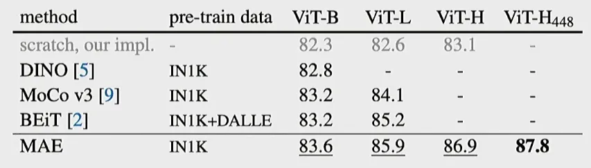
표에서는 ImageNet-1K로 사전 학습한 ViT-B의 MAE가 DINO·MoCo v3보다 높고, ViT-L에서는 MoCo v3보다 높다. BEiT는 추가로 DALL-E를 사용한 조건이므로 pretraining data가 동일한 비교는 아니다.

다만 reconstruction image가 눈으로 자연스러워 보이는 것과 representation quality는 같은 지표가 아니다. MAE 역시 linear probe와 downstream transfer 결과로 평가해야 한다.

Contrastive learning

Rotation, jigsaw, colorization과 MAE는 각각 회전 각도, patch 순서, 색, 가려진 pixel처럼 정해진 output을 맞히도록 학습한다. 하지만 좋은 feature를 얻기 위해 꼭 이런 output 자체를 복원할 필요는 없다. 같은 image를 다르게 변형한 두 view는 원본이 같고, 다른 image에서 온 view는 원본이 다르다는 관계도 label 없이 알 수 있다.

Contrastive learning은 이 관계를 학습 신호로 삼아 같은 image의 representation은 가깝게, 다른 image의 representation은 멀게 만든다. 다만 어떤 augmentation을 쓰고 positive·negative pair를 어떻게 구성할지는 여전히 설계해야 한다.

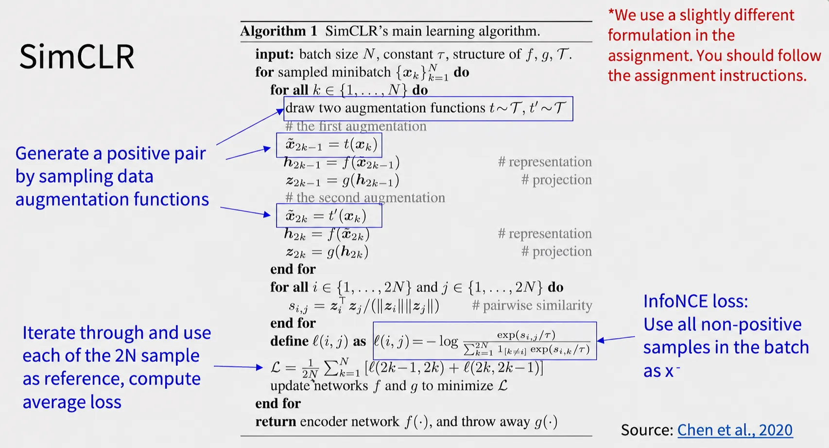
하나의 image $x_i$에 서로 다른 augmentation $t,t'$를 적용한 두 view를 positive pair로 만든다.

$$\tilde{x}_i = t(x_i)$$ $$\tilde{x}_i^+ = t'(x_i)$$

다른 image에서 나온 view는 negative sample로 사용한다. Reference sample을 $x$, 같은 image에서 만든 positive를 $x^+$, 다른 image에서 온 negative를 $x^-$라고 쓰면, encoder $f$가 학습해야 할 관계는 다음과 같다.

$$\operatorname{score}\left(f(x),f(x^+)\right) \gg \operatorname{score}\left(f(x),f(x^-)\right)$$

즉 positive pair의 score는 높이고 negative pair의 score는 낮춘다. 실제 구현에서는 encoder와 projection head를 차례로 통과시켜 embedding을 만들 수도 있다.

$$h_i = f_\theta(\tilde{x}_i)$$ $$z_i = g_\phi(h_i)$$

Similarity score $s$로는 보통 cosine similarity에 temperature $\tau$를 적용한다.

$$s(u,v) = \frac{u^Tv} {\lVert u\rVert_2\lVert v\rVert_2\tau}$$

$\tau$가 작으면 similarity 차이가 softmax에서 더 날카롭게 반영되고, 크면 distribution이 더 부드러워진다.

InfoNCE loss

InfoNCE는 Information Noise-Contrastive Estimation의 약자다. Positive를 여러 후보 중에서 구분하도록 학습시키는 contrastive loss이다.

Reference $x$마다 positive $x^+$ 하나와 negative $x^-_j$ $N-1$개가 있을 때, InfoNCE loss는 다음과 같다. 여기서 $f$는 비교할 embedding을 만드는 함수를 나타내며, projection head를 쓰는 경우에는 위의 $g_\phi\circ f_\theta$에 해당한다.

$$\mathcal{L}_{\text{InfoNCE}} = -\mathbb{E}_{x,x^+,x^-_{1:N-1}} \left[ \log \frac{ \exp\left(s(f(x),f(x^+))\right) }{ \exp\left(s(f(x),f(x^+))\right) + \sum_{j=1}^{N-1} \exp\left(s(f(x),f(x^-_j))\right) } \right]$$

이 식의 $N$은 positive 하나를 포함한 전체 후보 수다. 아래 SimCLR 절의 $N$은 batch에 들어 있는 원본 image 수이므로 구분해야 한다.

이 식은 여러 candidate 중 positive sample을 정답 class로 찾는 cross entropy로 볼 수 있다. Loss를 줄이려면 positive similarity는 커지고 negative similarity는 작아져야 한다.

InfoNCE는 일정한 sampling 가정 아래 positive pair의 embedding 사이 mutual information에 대한 lower bound를 제공한다. 위에서 정의한 전체 후보 수 $N$을 쓰면 슬라이드의 관계는 다음과 같다.

$$\operatorname{MI}\left[f(x),f(x^+)\right] - \log N \ge -\mathcal{L}_{\text{InfoNCE}}$$

따라서 InfoNCE loss를 낮추면 이 lower bound를 높일 수 있다. 다만 loss가 mutual information 자체와 완전히 같다는 뜻은 아니며, bound의 tightness는 negative sampling과 candidate 수에 영향을 받는다.

Negative sample이 많으면 positive를 더 어려운 후보들 사이에서 구분해야 하므로 representation이 좋아질 수 있다. 반면 실제로 같은 semantic class인 image를 negative로 취급하는 false negative가 생길 수 있고, 많은 negative를 저장하고 비교하는 memory와 compute 비용도 증가한다.

Contrastive Predictive Coding

Contrastive Predictive Coding, CPC는 sequence의 현재 context로 미래의 latent representation을 예측한다. Encoder가 각 input 구간을 latent $z_t$로 바꾸고 autoregressive model이 현재까지의 context $c_t$를 만든다.

$$z_t = g_{\text{enc}}(x_t)$$ $$c_t = g_{\text{ar}}(z_{\le t})$$

Future latent $z_{t+k}$가 positive이며 다른 sequence나 위치에서 뽑은 latent가 negative가 된다. InfoNCE는 후보들 사이에서 실제 future latent를 구분하도록 학습한다. Raw input을 직접 생성하는 대신 latent space에서 예측하므로 pixel이나 waveform의 세부 변동보다 시간적으로 유지되는 high-level structure에 집중할 수 있다.

CPC의 핵심은 contrastive objective를 사용해 representation 사이의 predictive information을 보존하는 것이다. 이후 SimCLR은 이 생각을 image augmentation으로 만든 두 view 사이의 instance discrimination 문제로 단순화하였다.

Representation collapse

Positive pair만 가깝게 만드는 objective를 아무 제약 없이 사용하면 모든 input을 같은 vector로 보내는 해가 가능하다.

$$f_\theta(x) = c \qquad \text{for all }x$$

이 경우 모든 positive pair의 거리는 0이지만 representation에는 input을 구분할 정보가 없다. 이를 representation collapse라고 한다.

Contrastive learning의 negative sample은 서로 다른 image의 embedding을 분리하므로 collapse를 직접 막는다. Negative를 사용하지 않는 방법은 stop-gradient, momentum teacher, predictor, centering, sharpening 등 다른 비대칭성과 regularization으로 collapse를 막아야 한다.

SimCLR

SimCLR은 별도의 memory bank나 momentum encoder 없이 augmentation, shared encoder, projection head, contrastive loss로 구성한 단순한 framework이다.

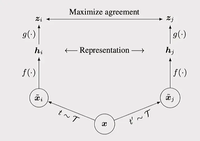
Batch에 original image가 $N$개 있으면 각 image에서 두 view를 만들어 총 $2N$개를 encoder에 넣는다. 한 view를 anchor로 볼 때 같은 original image의 다른 view 하나가 positive이고, 나머지 $2N-2$개 view가 negative이다.

$$\{x_1,\ldots,x_N\} \longrightarrow \{\tilde{x}_1,\ldots,\tilde{x}_{2N}\}$$

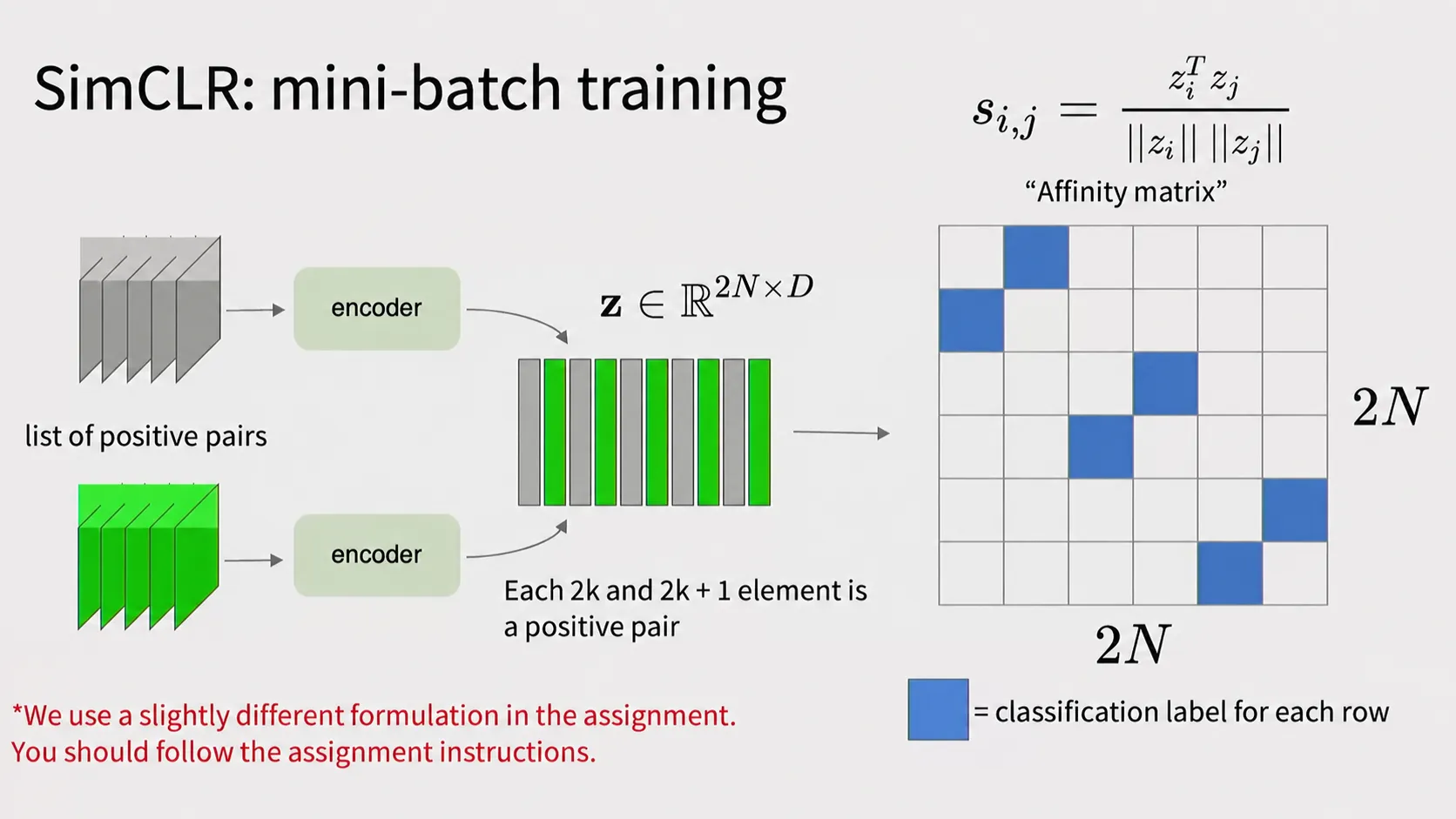
각 view를 shared encoder와 projection head에 통과시킨 embedding을 행으로 쌓으면 $Z\in\mathbb{R}^{2N\times D}$가 된다. 두 embedding의 cosine similarity $s_{i,j}=z_i^\top z_j/(\lVert z_i\rVert\lVert z_j\rVert)$를 계산하면 $2N\times2N$ affinity matrix가 만들어진다. 각 행에서 대각선은 자기 자신이므로 제외하고, 같은 원본 image에서 나온 다른 view의 칸이 positive 정답이다. 나머지 $2N-2$칸은 negative 후보가 된다. 그림은 짝을 $(2k,2k+1)$로 표시하지만, 아래 알고리즘의 $(2k-1,2k)$와 시작 인덱스만 다르다.

Positive pair $(i,j)$에 대한 NT-Xent loss는 다음과 같다.

$$\ell_{i,j} = -\log \frac{ \exp(\operatorname{sim}(z_i,z_j)/\tau) }{ \sum_{k=1}^{2N} \mathbf{1}_{[k\ne i]} \exp(\operatorname{sim}(z_i,z_k)/\tau) }$$

Pair의 양쪽을 각각 anchor로 사용하므로 최종 loss는 $2N$개 anchor에 대해 대칭적으로 평균한다.

$$\mathcal{L}_{\text{SimCLR}} = \frac{1}{2N} \sum_{(i,j)} \left( \ell_{i,j} + \ell_{j,i} \right)$$

여기서 합은 batch의 $N$개 positive pair에 대해 계산한다.

%% title: SimCLR의 Positive Pair와 In-Batch Negative
%% caption: 같은 image의 두 augmentation은 positive pair가 되고, batch의 다른 image view는 negative가 된다. Shared encoder와 projection head를 통과한 embedding에 InfoNCE loss를 적용한다.
flowchart LR
    image["Image xᵢ"] --> aug1["Random Augmentation t"]
    image --> aug2["Random Augmentation t'"]
    aug1 --> enc1["Shared Encoder fθ"]
    aug2 --> enc2["Shared Encoder fθ"]
    enc1 --> proj1["Projection Head gφ<br/>zᵢ"]
    enc2 --> proj2["Projection Head gφ<br/>zᵢ⁺"]
    proj1 --> positive["Positive Similarity ↑"]
    proj2 --> positive
    negatives["Other Batch Embeddings<br/>zₖ"] --> contrast["InfoNCE Softmax"]
    positive --> contrast
    contrast --> objective["positive 가깝게<br/>negatives 멀게"]

Augmentation이 정의하는 invariance

SimCLR에서 positive pair는 ground-truth semantic label이 아니라 augmentation으로 결정된다. 따라서 augmentation은 model이 어떤 변화에 invariant해야 하는지를 정의한다.

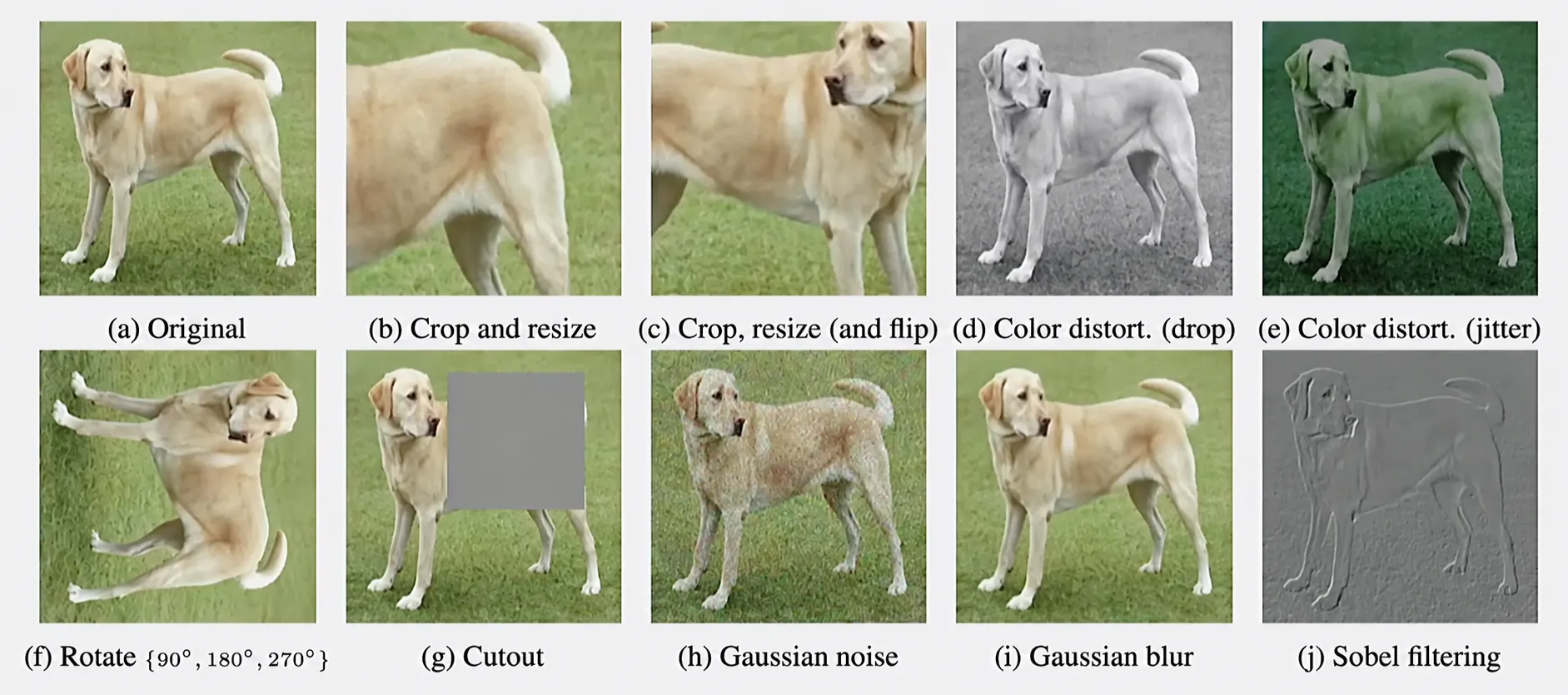
그림은 가능한 image augmentation의 예시이며, 모든 변환을 SimCLR에서 반드시 함께 사용하는 것은 아니다.

대표적인 augmentation은 다음과 같다.

• Random resized crop
• Horizontal flip
• Strong color jitter
• Random grayscale
• Gaussian blur

같은 object가 crop, color, blur가 달라도 같은 representation을 가져야 한다고 학습하는 것이다. 특히 random crop과 color distortion의 조합이 중요하다. Crop만 사용하면 model이 color histogram 같은 쉬운 단서로 같은 image를 찾을 수 있고, color distortion만 사용하면 spatial layout을 그대로 비교할 수 있다. 둘을 함께 사용하면 더 semantic한 feature가 필요하다.

하지만 invariance는 무조건 많을수록 좋은 것이 아니다. Color가 downstream label에 중요한 fine-grained task라면 지나친 color jitter가 필요한 정보를 제거할 수 있다. Augmentation은 downstream task에서 보존해야 할 요소와 무시해도 될 요소를 고려해 선택해야 한다.

Projection head를 따로 두는 이유

SimCLR은 encoder representation $h$ 위에 작은 nonlinear MLP $g$를 두고 contrastive loss는 projection $z=g(h)$에 적용한다. Downstream task에는 $z$보다 projection 이전의 $h$를 사용한다.

Contrastive objective는 augmentation에 대한 invariance를 강하게 요구한다. 이 과정에서 color, exact position처럼 downstream에서는 유용할 수 있는 정보까지 $z$에서 버릴 수 있다. Projection head가 contrastive objective에 특화된 공간을 따로 제공하면 encoder representation $h$에는 더 많은 정보가 남을 수 있다.

따라서 pretraining loss가 직접 적용되는 vector와 downstream에 사용하는 vector가 반드시 같을 필요는 없다.

SimCLR과 batch size

SimCLR은 batch 안의 다른 view를 negative로 사용하므로 batch size가 커질수록 한 anchor가 보는 negative 수가 늘어난다.

$$N_{\text{negative}} = 2N-2$$

Encoder output은 anchor를 포함해 총 $2N$개다. 한 view를 anchor로 잡으면 자기 자신을 제외한 $2N-1$개가 비교 대상이고, 그중 같은 원본에서 온 다른 view 하나가 positive이므로 negative는 $(2N-1)-1=2N-2$개다. 예를 들어 원본 image가 3개라면 $A_1,A_2,B_1,B_2,C_1,C_2$의 여섯 view가 생긴다. $A_1$을 anchor로 잡으면 $A_2$가 positive이고 $B_1,B_2,C_1,C_2$의 네 개가 negative다.

이는 memory bank 없이 많은 negative를 얻는 단순한 방법이지만, 매우 큰 batch와 accelerator memory가 필요하다. Distributed training에서는 여러 device의 embedding을 all-gather해 global batch의 negative로 사용할 수 있으며, 이때 representation learning 성능과 communication cost가 함께 증가한다.

SimCLR의 linear evaluation

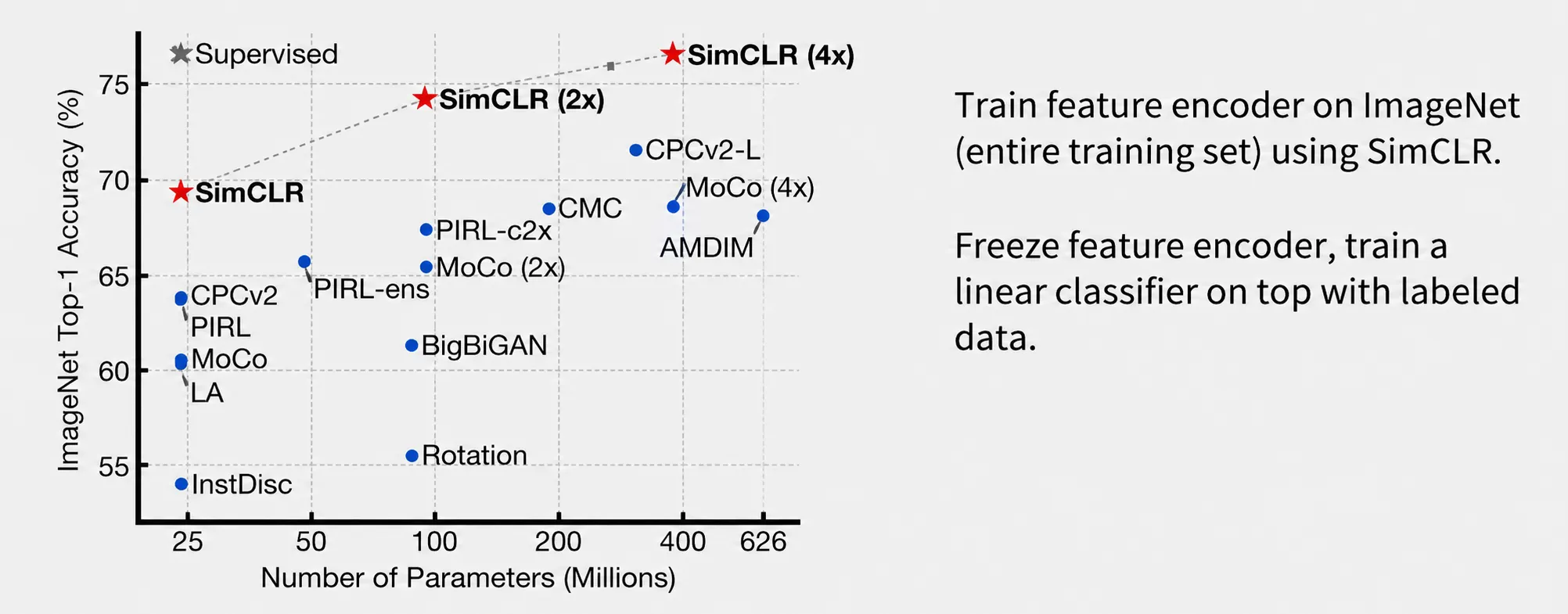
ImageNet 전체 학습 이미지로 encoder를 label 없이 pretrain한 뒤 encoder를 고정하고, label이 있는 데이터로 linear classifier만 학습해 feature의 유용성을 평가한다. 그래프의 x축은 파라미터 수, y축은 ImageNet Top-1 정확도다. SimCLR은 모델 규모가 커질수록 정확도가 높아지는 경향을 보이며, 이는 pretext loss 자체보다 학습된 representation의 downstream 성능을 확인하는 평가다.

MoCo의 queue와 momentum encoder

Momentum Contrast, MoCo는 이전 minibatch에서 만든 key embedding을 queue에 저장해 negative로 재사용한다. 새 key를 넣고 가장 오래된 key를 빼는 FIFO 방식이므로, 현재 batch가 작아도 query 하나를 queue의 수많은 negative와 비교할 수 있다. 즉 negative 수를 batch size와 분리한다.

하지만 저장된 key는 과거 encoder로 계산한 값이다. Encoder가 매 step 크게 바뀌면 새 query와 오래된 key의 유사도를 일관된 기준으로 비교하기 어렵다. MoCo는 gradient로 학습하는 query encoder와, 그 parameter를 천천히 따라가는 momentum key encoder를 함께 써서 queue의 key들이 비교적 안정적인 공간에 머물게 한다.

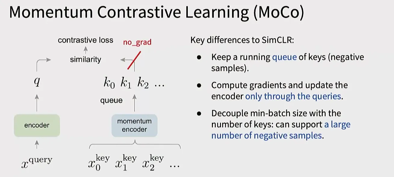
그림에서 $q$와 대응하는 $k_0$는 positive pair이고, queue의 $k_1,k_2,\ldots$는 negative 후보이다. Loss의 gradient는 query encoder로만 전달되고, key encoder는 아래 momentum 식으로 갱신한다. 따라서 minibatch가 작아도 queue에 쌓인 많은 negative를 비교할 수 있다.

MoCo에는 두 encoder가 있다.

• Query encoder $f_q$는 backpropagation으로 학습한다.
• Key encoder $f_k$는 query encoder parameter의 exponential moving average로 update한다.

Query encoder parameter를 $\theta_q$, key encoder parameter를 $\theta_k$라고 하면 다음과 같다.

$$\theta_k \leftarrow m\theta_k + (1-m)\theta_q$$

$m$은 보통 1에 가까운 momentum coefficient이다. 예를 들어 $m=0.999$이면 이전 key encoder parameter를 $99.9\%$ 유지하고 현재 query encoder parameter를 $0.1\%$만 반영하므로 key encoder가 천천히 변한다.

Embedding을 정규화하고 queue에 negative key가 $K$개 있을 때, query 하나에 대한 contrastive loss는 다음과 같다.

$$\mathcal{L}_{q} = -\log \frac{\exp(q^{\top}k^{+}/\tau)} {\exp(q^{\top}k^{+}/\tau)+\sum_{i=1}^{K}\exp(q^{\top}k_i^{-}/\tau)}$$

여기서 $k^{+}=k_0$는 현재 query의 positive key, $k_i^{-}$는 queue에서 가져온 negative key, $\tau$는 temperature이다.

한 iteration은 다음 순서로 볼 수 있다.

1. Current view를 query encoder에 넣어 query $q$를 만든다.
2. Positive view를 key encoder에 넣어 positive key $k^+$를 만든다.
3. Queue에 저장된 key들을 negative로 사용해 InfoNCE loss를 계산한다.
4. Query encoder를 backpropagation으로 update한다.
5. Key encoder를 momentum update한다.
6. Current minibatch의 key를 enqueue하고 가장 오래된 key를 dequeue한다.

Queue의 old key는 과거 parameter로 계산되었고 computation graph도 이미 사라졌으므로 그 key를 통해 backpropagation할 수 없다.

MoCo v2는 MoCo의 queue와 momentum encoder에 SimCLR에서 효과적이었던 stronger augmentation과 MLP projection head를 결합한다.

%% title: MoCo의 Momentum Encoder와 Negative Queue
%% caption: Query encoder는 gradient로 학습하고 key encoder는 query parameter의 moving average로 갱신한다. 과거 key를 queue에 저장해 batch 크기보다 많은 negative를 사용한다.
flowchart LR
    viewq["Query View"] --> fq["Query Encoder f_q"]
    viewk["Key View"] --> fk["Momentum Key Encoder f_k"]
    fq --> q["Query q"]
    fk --> kplus["Positive Key k⁺"]
    queue["FIFO Queue<br/>Past Keys"] --> loss["Contrastive Loss"]
    q --> loss
    kplus --> loss
    fq -. "EMA parameter update" .-> fk
    kplus --> enqueue["Enqueue New Key"]
    enqueue --> queue

SimCLR과 MoCo 비교

항목	SimCLR	MoCo
Negative source	Current batch의 다른 view	Queue의 current와 previous key
Negative 수	Batch size에 직접 의존	Queue size로 조절
Encoder	Shared encoder 하나	Query encoder와 momentum key encoder
Parameter update	Backpropagation	Query는 backpropagation, key는 EMA
주요 장점	구조가 단순함	작은 batch에서도 많은 negative 사용 가능
주요 비용	큰 batch와 device memory	Queue 관리와 두 encoder forward

두 방법의 핵심 objective는 같은 image의 두 view를 가깝게 하고 다른 image의 representation을 구분하는 것이다. 차이는 negative dictionary를 어떻게 구성하고 시간에 따라 일관되게 유지하는지에 있다.

Negative가 없는 teacher-student 방식

DINO 같은 방식은 explicit negative 없이 서로 다른 augmentation의 output distribution을 맞춘다. Student는 gradient로 학습하고 teacher는 student parameter의 exponential moving average로 update한다.

$$\theta_{\text{teacher}} \leftarrow m\theta_{\text{teacher}} + (1-m)\theta_{\text{student}}$$

Teacher output에는 stop-gradient를 적용하고, centering과 temperature sharpening으로 모든 sample이 같은 distribution을 내는 collapse를 억제한다. Contrastive method가 negative와의 상대적인 분리로 representation을 학습한다면, teacher-student method는 두 network와 두 view 사이의 비대칭적인 consistency objective를 사용한다.

MAE, SimCLR, MoCo, DINO는 모두 label 없이 encoder를 pretrain하지만 학습 신호가 다르다.

계열	학습 target	Model이 배워야 하는 것
Handcrafted pretext	Rotation, 위치, 색 등	사람이 정한 transformation의 구조
Masked reconstruction	가려진 original pixel	Visible context에서 missing content 추론
Contrastive learning	Positive와 negative 관계	같은 instance의 view는 모으고 다른 instance는 분리
Teacher-student	Teacher의 output distribution	서로 다른 view에서 일관된 representation

Self-supervised learning에서 확인할 trade-off

Self-supervised method를 비교할 때 downstream accuracy 하나만 볼 수는 없다.

• Data scale: 더 많은 unlabeled data를 사용할 때 성능이 얼마나 증가하는가?
• Label efficiency: $1\%$, $10\%$처럼 label이 적을 때 얼마나 잘 transfer되는가?
• Compute: Pretraining FLOPs와 accelerator 수가 얼마나 필요한가?
• Memory: Large batch, queue, decoder가 요구하는 memory가 얼마인가?
• Architecture: CNN과 ViT 중 어떤 encoder에 잘 맞는가?
• Evaluation protocol: Linear probe인지 full fine-tuning인지 같은 조건인가?
• Robustness: Domain shift와 corruption에서도 feature가 유지되는가?
• Invariance: Augmentation이 downstream에 필요한 정보를 없애지는 않는가?

Pretraining dataset, encoder size, training epoch, augmentation, optimizer가 다르면 method 자체의 차이와 scale의 효과를 분리하기 어렵다. 따라서 논문 수치를 비교할 때는 evaluation protocol과 compute budget을 함께 봐야 한다.

과제에서 확인할 것

SimCLR loss 구현

• Batch의 $N$개 image에서 두 view씩 만들어 embedding이 $2N$개가 되는지 확인한다.
• 각 anchor의 positive index가 같은 source image의 다른 view를 정확히 가리키는지 확인한다.
• 자기 자신과의 similarity가 denominator에서 제외되는지 확인한다.
• Cosine similarity를 계산하기 전에 embedding을 L2 normalize하는지 확인한다.
• Temperature $\tau$가 logit 전체에 같은 방식으로 적용되는지 확인한다.
• Pair의 양쪽을 anchor로 사용하는 symmetric loss인지 확인한다.
• Assignment notebook의 loss 정의와 index 배치가 위의 일반식과 조금 다를 수 있으므로 notebook의 convention을 우선한다.

수치 안정성

InfoNCE는 softmax cross entropy이므로 similarity logit이 클 때 그대로 exponentiation하면 overflow가 생길 수 있다. 실제 구현에서는 row별 maximum을 빼거나 logsumexp를 사용해 계산해야 한다.

$$\log \sum_j e^{s_j} = m + \log \sum_j e^{s_j-m}$$

여기서 $m=\max_j s_j$이다. Maximum을 빼도 softmax probability는 변하지 않는다.

Representation 평가

• Pretraining loss만 보고 encoder가 좋아졌다고 판단하지 않는다.
• Encoder를 freeze한 linear probe와 encoder까지 update하는 fine-tuning을 구분한다.
• Augmentation strength를 바꾸었을 때 positive pair가 지나치게 쉬워지거나 semantic content가 사라지지 않는지 확인한다.
• Projection head의 output $z$와 encoder output $h$ 중 어느 feature를 downstream에 사용하는지 확인한다.
• Batch size를 바꿀 때 negative 수, learning rate, distributed all-gather 조건도 함께 달라지는지 확인한다.

MAE를 구현하거나 실험할 때

• Encoder에는 visible patch만 들어가는지 확인한다.
• Mask token이 encoder가 아니라 decoder input에 추가되는지 확인한다.
• Positional embedding을 사용해 shuffled visible token과 mask token의 원래 위치를 복원하는지 확인한다.
• Reconstruction loss가 모든 patch가 아니라 masked patch에 대해서만 계산되는지 확인한다.
• Mask ratio를 바꾸었을 때 task difficulty와 encoder compute가 함께 변한다는 점을 확인한다.
• Pretraining 후 decoder를 제거하고 encoder만 downstream task에 사용하는지 확인한다.