목차

Overview

softmaxloss 에 대해서 이해하고, svm loss와 softmaxloss의 차이를 확인하고, SGD를 적용해서 훈련을 수행하고, 검증 데이터로 하이퍼파라미터 결정하기

핵심 아이디어

softmaxloss 는 모델이 정답 클래스에 얼마나 높은 확률을 부여했는지를 기준으로 손실을 계산하는 방법이다.

• score를 softmax로 변환하여 각 클래스의 확률을 계산
• 정답 클래스의 확률이 1에 가까울수록 loss가 작아짐
• SVM loss와 달리 margin을 넘겨도 정답 확률을 더 키우는 방향으로 계속 학습

수식:
logit(점수):

$$p_{i,k} = \frac{\exp(s_{i,k})} {\sum_j \exp(s_{i,j})}$$

loss:

$$L_i = -\log p_{i,y_i}$$

full loss:

$$L = \frac{1}{N} \sum_{i=1}^{N} -\log p_{i,y_i} + \lambda \sum W^2$$

loss range:

$$0 \leq L_i < \infty$$ $$p_{i,y_i} \rightarrow 1 \quad \Rightarrow \quad L_i \rightarrow 0$$ $$p_{i,y_i} \rightarrow 0 \quad \Rightarrow \quad L_i \rightarrow \infty$$

구현

loop -> vectorized

Inputs:
    - W: A numpy array of shape (D, C) containing weights.
    - X: A numpy array of shape (N, D) containing a minibatch of data.
    - y: A numpy array of shape (N,) containing training labels; y[i] = c means
      that X[i] has label c, where 0 <= c < C.
    - reg: (float) regularization strength

loop:

• 샘플 갯수 N 만큼 순회하며, 입력 X[i]와 가중치 W를 내적하여 score 산출
  (D, ) (D, C) => (C, )

• score 기반으로 softmax 산출

• loss -= logp[y[i]] 처리
  y는 shape이 (N, )인 정답 label 배열, y[i]는 i번째 샘플의 정답 클래스 index인 scalar
  logp[y[i]]는 정답 클래스의 log probability를 의미하며, loss에는 $-\log p_{y_i}$가 더해짐

• dscore = p.copy()로 softmax probability vector를 복사 이때 dscore의 shape은 (C, )

• dscore[y[i]] -= 1은 정답 클래스 위치에만 -1
  one-hot vector t에 대해 softmax loss의 gradient인 $p - t$를 구현

  $$\frac{\partial L}{s} = p-t$$

• np.outer(X[i], dscore)는 입력 feature vector와 score gradient의 outer product를 계산
  shape은 (D, ) outer (C, ) => (D, C)가 되며, 이는 현재 샘플 하나가 만드는 dW
  모든 샘플의 기여도를 누적 후 1/N

def softmax_loss_naive(W, X, y, reg):
    loss = 0.0
    dW = np.zeros_like(W)

    num_classes = W.shape[1] # C
    num_train = X.shape[0] # N
    for i in range(num_train):
        scores = X[i].dot(W) # (D,) (D,C) -> (C,)

        scores -= np.max(scores)
        p = np.exp(scores)
        p /= p.sum()
        logp = np.log(p)

        loss -= logp[y[i]]

        dscore = p.copy()
        dscore[y[i]] -= 1
        dW += np.outer(X[i], dscore)

    loss = loss / num_train + reg * np.sum(W * W)

    dW = dW / num_train + 2 * reg * W

    return loss, dW

vectorized:

• score를 X @ W 로 바로 계산
• softmax 계산 후 정답 라벨을 이용해 정답 확률만 가져옴
• dW 를 chain rule 공식으로 바로 계산

def softmax_loss_vectorized(W, X, y, reg):
    loss = 0.0
    dW = np.zeros_like(W)

    num_train = X.shape[0] # N
    
    scores = X @ W # (N, C)

    scores -= np.max(scores, axis=1, keepdims=True)

    p = np.exp(scores)
    p /= np.sum(p, axis=1, keepdims=True)

    logp = np.log(p)

    correct_logp = logp[np.arange(num_train), y] # (N, )

    loss = -np.sum(correct_logp) / num_train

    loss += reg * np.sum(W * W)

    dscore = p.copy() # (N, C)

    dscore[np.arange(num_train), y] -= 1
    
    # X(N, D), dscore(N, C)
    dW = X.T @ dscore

    dW = dW / num_train + 2 * W * reg

    return loss, dW

---

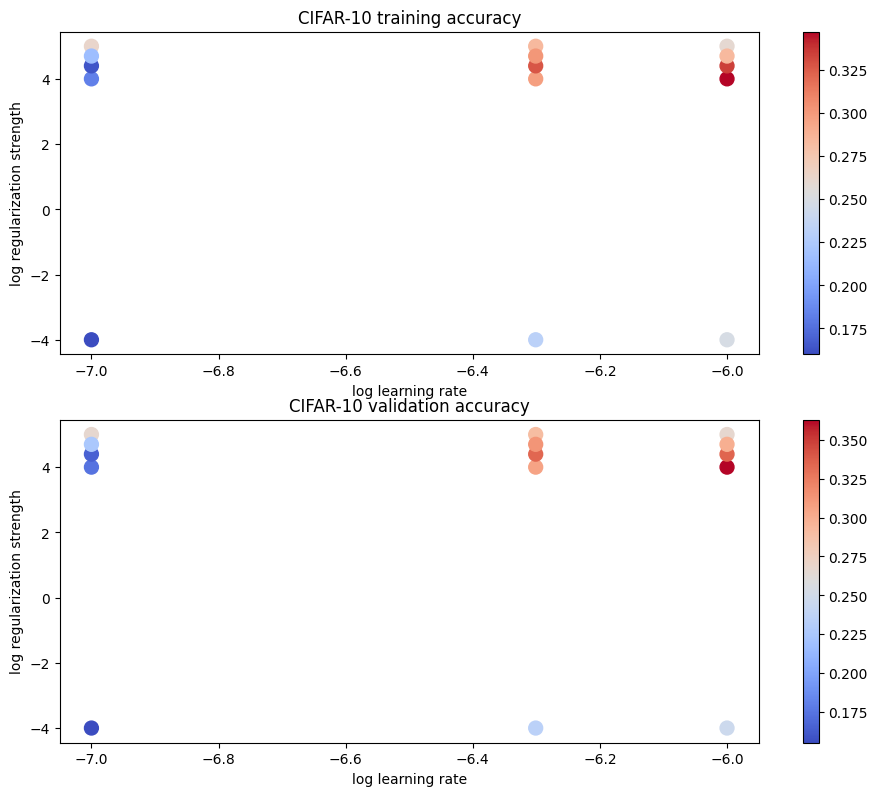
검증 데이터로 하이퍼파라미터 결정

• learning_rates, regularization_strengths 결정

learning_rates = [1e-7, 5e-7, 1e-6]
regularization_strengths = [1e4, 1e05, 2.5e4, 5e4]

num_iter = 150

for lr in learning_rates:
  for reg in regularization_strengths:
    model = Softmax()
    
    model.train(X_train, y_train, lr, reg, num_iter)

    train_pred = model.predict(X_train)

    train_acc = np.sum(train_pred == y_train) / y_train.shape[0]

    val_pred = model.predict(X_val)

    val_acc = np.sum(val_pred == y_val) / y_val.shape[0]

    results[(lr, reg)] = (train_acc, val_acc)

    if val_acc > best_val:
      best_val = val_acc
      best_softmax = model

lr 1.000000e-06 reg 1.000000e+04 train accuracy: 0.347000 val accuracy: 0.363000
during cross-validation: 0.363000

• lr: 1e-6 에서 전반적으로 acc > 0.3 확인 후 reg 범위를 1e4 ~ 1e6까지 조정

추가 개념들

SVM loss와 gradcheck discrepancy

SVM loss는 hinge loss 형태라서 margin boundary에서 미분 불가능한 지점이 생긴다.

$$L_i = \sum_{j \neq y_i} \max(0, s_j - s_{y_i} + \Delta)$$

문제가 생기는 지점은 다음과 같다.

$$s_j - s_{y_i} + \Delta = 0$$

이 지점에서는 $\max(0, x)$의 꺾이는 부분 때문에 gradient가 명확하게 하나로 정해지지 않는다.

간단한 1차원 예시는 다음과 같다.

$$f(x) = \max(0, x)$$ $$x = 0$$

이때 numerical gradient는 centered difference 때문에 대략 $\frac{1}{2}$가 나올 수 있지만, analytic gradient는 구현에 따라 $0$ 또는 $1$로 처리될 수 있다.

따라서 SVM gradcheck에서 일부 dimension이 가끔 맞지 않는 것은 큰 문제가 아니다.
margin $\Delta$를 바꾸면 boundary 위치가 바뀌므로, data point가 boundary 근처에 많이 걸릴수록 discrepancy가 더 자주 발생할 수 있다.

---

SVM loss와 Softmax loss의 차이

SVM loss는 margin 기반 loss라서, 정답 class score가 모든 오답 class score보다 margin $\Delta$ 이상 크면 loss가 0이 된다.

$$L_i^{SVM} = \sum_{j \neq y_i} \max(0, s_j - s_{y_i} + \Delta)$$ $$s_{y_i} \geq s_j + \Delta \quad \forall j \neq y_i \Rightarrow L_i^{SVM}=0$$

반면 Softmax loss는 정답 class probability가 1에 가까워질수록 작아지지만, 정확히 1이 아니면 loss가 양수이다.

$$L_i^{Softmax} = -\log p_{i,y_i}$$ $$0 < p_{i,y_i} < 1 \Rightarrow L_i^{Softmax} > 0$$

따라서 SVM loss는 margin 조건을 만족하면 더 이상 loss가 줄어들지 않지만, Softmax loss는 정답 class probability를 계속 더 크게 만드는 방향으로 학습된다.

헷갈렷던 포인트

loop 구현에서 형상에 맞춰서 outer product 수행:
모든 feature D 와 모든 class C 의 조합을 만들기 위해서 외적 사용, dW에 누적

Linear classifier backprop chain rule

Forward:

$$S = XW$$ $$X \in \mathbb{R}^{N \times D}, \quad W \in \mathbb{R}^{D \times C}, \quad S \in \mathbb{R}^{N \times C}$$

Upstream gradient:

$$dS = \frac{\partial L}{\partial S}$$ $$dS \in \mathbb{R}^{N \times C}$$

Gradient w.r.t. weight:

$$dW = \frac{\partial L}{\partial W} = X^T dS$$ $$X^T \in \mathbb{R}^{D \times N}, \quad dS \in \mathbb{R}^{N \times C} \Rightarrow dW \in \mathbb{R}^{D \times C}$$

Gradient w.r.t. input:

$$dX = \frac{\partial L}{\partial X} = dS W^T$$ $$dS \in \mathbb{R}^{N \times C}, \quad W^T \in \mathbb{R}^{C \times D} \Rightarrow dX \in \mathbb{R}^{N \times D}$$

Single sample case:

$$s_i = x_i W$$ $$dW_i = \frac{\partial L_i}{\partial W} = x_i^T ds_i$$ $$x_i^T \in \mathbb{R}^{D \times 1}, \quad ds_i \in \mathbb{R}^{1 \times C} \Rightarrow dW_i \in \mathbb{R}^{D \times C}$$

Softmax loss case:

$$ds_i = \frac{\partial L_i}{\partial s_i} = p_i - t_i$$

Therefore:

$$dW_i = x_i^T (p_i - t_i)$$

Batch average:

$$dW = \frac{1}{N} X^T (P - T)$$

With regularization:

$$L = L_{data} + \lambda \sum W^2$$ $$dW = \frac{1}{N} X^T (P - T) + 2\lambda W$$