한빛미디어의 <밑바닥부터 시작하는 딥러닝 2>를 요약 정리한 글이다.

Transformer의 출발점이 된 논문은 Attention is All You Need(2017)이다.

Attention의 가장 간단한 직관은 다음과 같다.

Decoder의 현재 은닉 상태 $h$와 Encoder의 전체 은닉 상태 $\mathrm{hs}$를 비교하여 score를 구하고, 이 score를 softmax로 정규화해 attention weight $a$를 만든 뒤, $\mathrm{hs}$와 $a$의 가중합으로 attention context vector를 만든다.

Attention Context Vector는 Decoder의 현재 시점에 필요한 입력 문맥을 가중합으로 요약한 벡터이다.

seq2seq의 문제점

기본 seq2seq는 Encoder가 입력 시계열 데이터를 읽고, 그 정보를 Decoder로 전달하는 구조이다.

이때 Encoder가 Decoder로 넘기는 정보는 고정 길이 벡터이다.

기존 구조에서는 LSTM의 마지막 은닉 상태 $\mathrm{h}_T$만 Decoder로 전달했다.

즉 입력 문장이 길어지더라도 Encoder는 마지막 은닉 상태 하나에 전체 입력 문장의 정보를 압축해야 한다.

이 구조는 다음 한계를 가진다.

• Encoder가 시계열 데이터를 인코딩한다.
• 인코딩된 정보는 Decoder로 전달된다.
• 이때 전달되는 정보는 고정 길이 벡터이다.
• LSTM의 마지막 은닉 상태 $\mathrm{h}_T$만 사용한다.
• 따라서 구조적으로 표현력이 제한된다.

입력 문장이 짧으면 마지막 은닉 상태 하나로도 어느 정도 정보를 담을 수 있다.

하지만 입력 문장이 길어지면 앞쪽 단어의 정보가 충분히 보존되지 못할 수 있다.

Attention은 이 문제를 완화하기 위해 Encoder의 마지막 은닉 상태 하나만 사용하는 대신, Encoder의 모든 시점 은닉 상태를 활용한다.

seq2seq 개선 방향

개선된 구조에서는 LSTM 각 시점의 은닉 상태 벡터 $\mathrm{hs}$를 모두 사용한다.

구현 관점에서는 return_sequences=True로 전체 시점의 hidden state를 반환하게 만든다고 볼 수 있다.

여기서 $\mathrm{hs}$는 입력 단어 수만큼의 벡터를 포함한다.

예를 들어 입력 단어가 $T$개라면 $\mathrm{hs}$는 다음과 같은 형태를 가진다.

$$\mathrm{hs} = \left[ h_1, h_2, \dots, h_T \right]$$

각 벡터 hs[i]에는 입력 단어 input_word[i]에 대한 정보가 가장 많이 포함된다.

다만 RNN 계열 구조에서는 hs[i]에 i 이전 시점의 단어 정보가 함께 포함된다.

반대로 i 이후 시점의 단어 정보까지 반영하려면 양방향 RNN을 사용하기도 한다.

Decoder 개선 1: Encoder의 전체 hs 사용

Attention을 적용하려면 Decoder가 Encoder의 마지막 hidden state hs[-1]만 받는 것이 아니라, Encoder의 전체 hidden states hs를 받을 수 있어야 한다.

기존 구조에서 Encoder의 마지막 시점 은닉 상태 hs[:, -1, :]는 Decoder의 첫 번째 LSTM 계층에 전달된다.

Attention 구조에서는 이 흐름은 유지하되, 추가로 Encoder의 전체 hs도 Decoder 내부에서 활용한다.

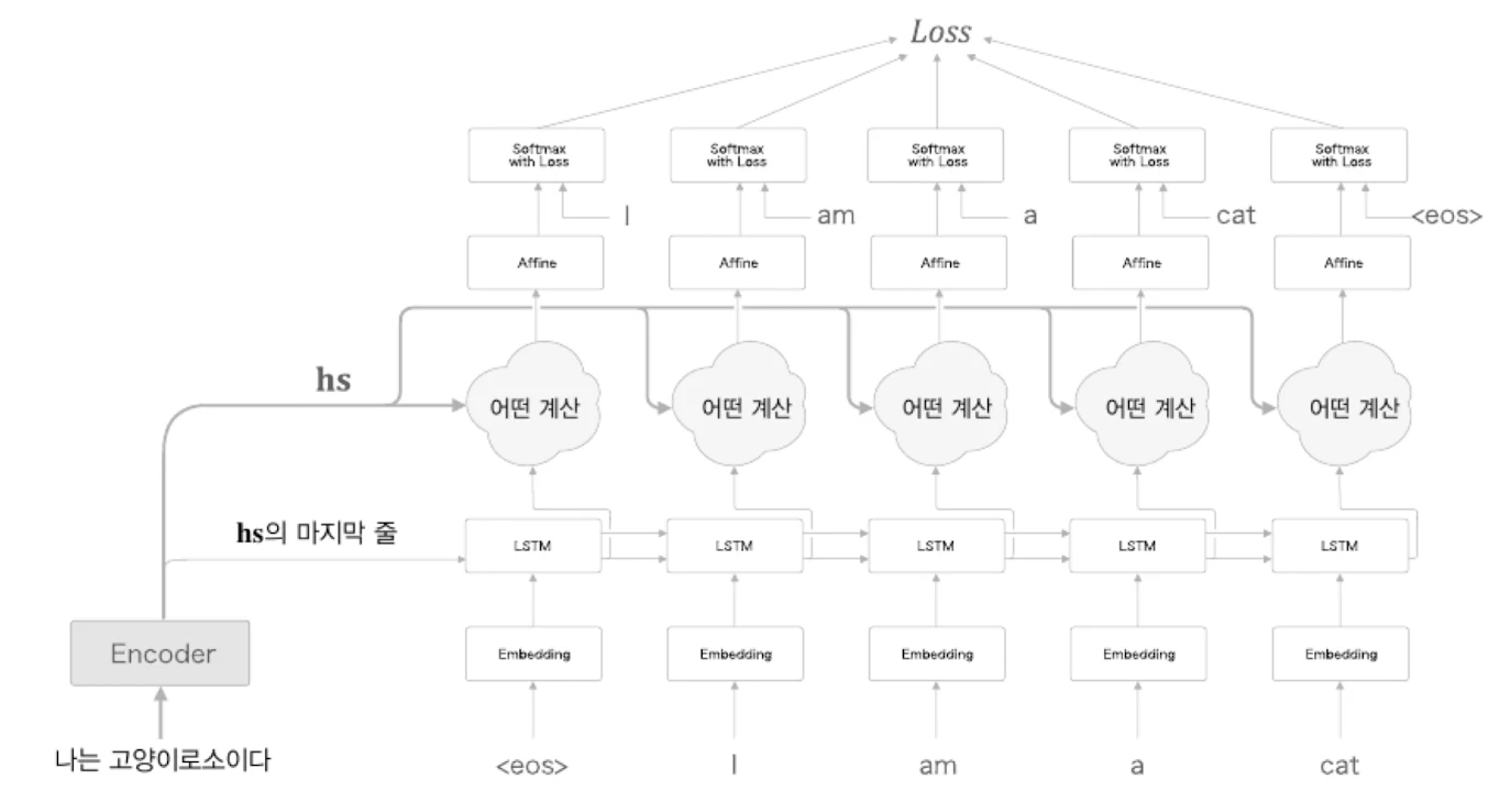
위 구조에서 새로 추가된 Attention 관련 계층은 두 개의 입력을 받는다.

• Encoder로부터 전달받은 전체 hs
• 각 시각별 Decoder LSTM의 은닉 상태

이 신경망이 수행하는 일은 단어들의 alignment를 추출하는 것이다.

Alignment

Alignment는 단어 또는 문구 사이의 대응 관계를 나타내는 정보이다.

예를 들어 번역 문제에서는 다음과 같은 대응 관계가 필요하다.

• 나는 I와 대응된다.
• 고양이는 cat과 대응된다.

과거에는 이런 대응 관계를 사람이 직접 설계하거나 수작업으로 다루는 경우가 많았다.

Attention은 이 alignment를 데이터로부터 자동으로 학습하도록 만든다.

Attention의 목표는 다음과 같다.

도착어 단어와 대응 관계에 있는 출발어 단어의 정보를 골라내고, 그 정보를 이용하여 번역을 수행하는 것이다.

즉 필요한 정보에만 주목하여, 그 정보로부터 시계열 변환을 수행하는 방식이다.

seq2seq에서는 각 시각에서 Decoder에 입력된 단어와 대응 관계인 입력 단어의 벡터를 $\mathrm{hs}$에서 골라내고 싶다.

하지만 여기서 문제가 생긴다.

hs의 여러 벡터 중 하나를 직접 선택하는 연산은 미분할 수 없다.

즉 “여러 개 중 하나를 고르는 작업”은 오차역전파법으로 학습하기 어렵다.

그래서 Attention은 하나만 선택하지 않는다.

대신 모든 벡터를 선택하되, 각 벡터에 중요도를 나타내는 가중치 $a$를 부여한다.

선택 대신 가중합 사용

Attention은 특정 시점에서 하나의 벡터만 고르는 대신, 모든 Encoder hidden states를 사용한다.

대신 각 단어별 중요도를 나타내는 가중치 $a$를 도입한다.

이 가중치 $a$는 일종의 확률분포이다.

각 시점의 가중치를 모두 더하면 1이 되며, 값이 클수록 해당 입력 단어가 현재 Decoder 시점에 더 중요하다는 뜻이다.

이후 Encoder hidden states hs와 attention weight a의 가중합을 통해 맥락 벡터 c를 계산한다.

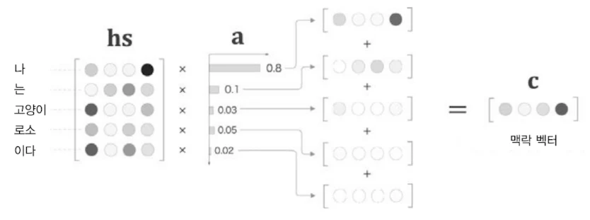
맥락 벡터 c는 현재 시각의 변환, 예를 들어 번역에서 현재 출력 단어를 생성하는 데 필요한 정보를 담는다.

만약 현재 출력해야 하는 단어가 I이고, 입력 문장의 나에 해당하는 hidden state가 중요하다면, 나에 대응되는 위치의 attention weight가 크게 학습된다.

이때 맥락 벡터 c에는 나 벡터의 성분이 많이 포함된다.

즉 나를 직접 선택하는 작업을 미분 가능한 가중합으로 대체한 것이다.

Attention 직관

Attention은 매 시점마다 Encoder의 전체 hidden states hs와 Decoder의 현재 hidden state h를 비교한다.

이 비교는 보통 유사도 score를 계산하는 방식으로 이루어진다.

현재 Decoder가 출력하려는 단어와 입력 문장의 어떤 부분이 가장 관련이 높은지 score를 구하고, 이를 softmax로 정규화하면 attention weight가 된다.

전체 흐름은 다음과 같다.

Encoder hidden states hs
Decoder current hidden state h
→ similarity score s
→ softmax
→ attention weight a
→ weighted sum
→ context vector c

가중합 구현 예제

먼저 미니배치를 고려하지 않는 간단한 예제를 보자.

T, H = 5, 4
hs = np.random.randn(T, H)
a = np.array([0.8, 0.1, 0.03, 0.05, 0.02])
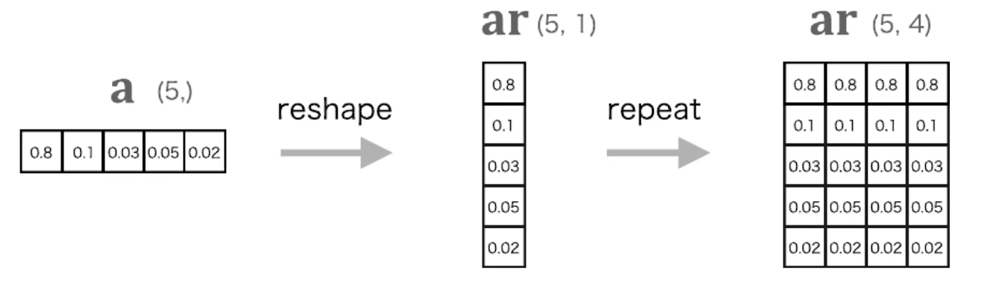
ar = a.reshape(5, 1).repeat(4, axis=1)

print(ar.shape)
# (5, 4)

t = hs * ar
print(t.shape)
# (5, 4)

c = np.sum(t, axis=0)
print(c.shape)
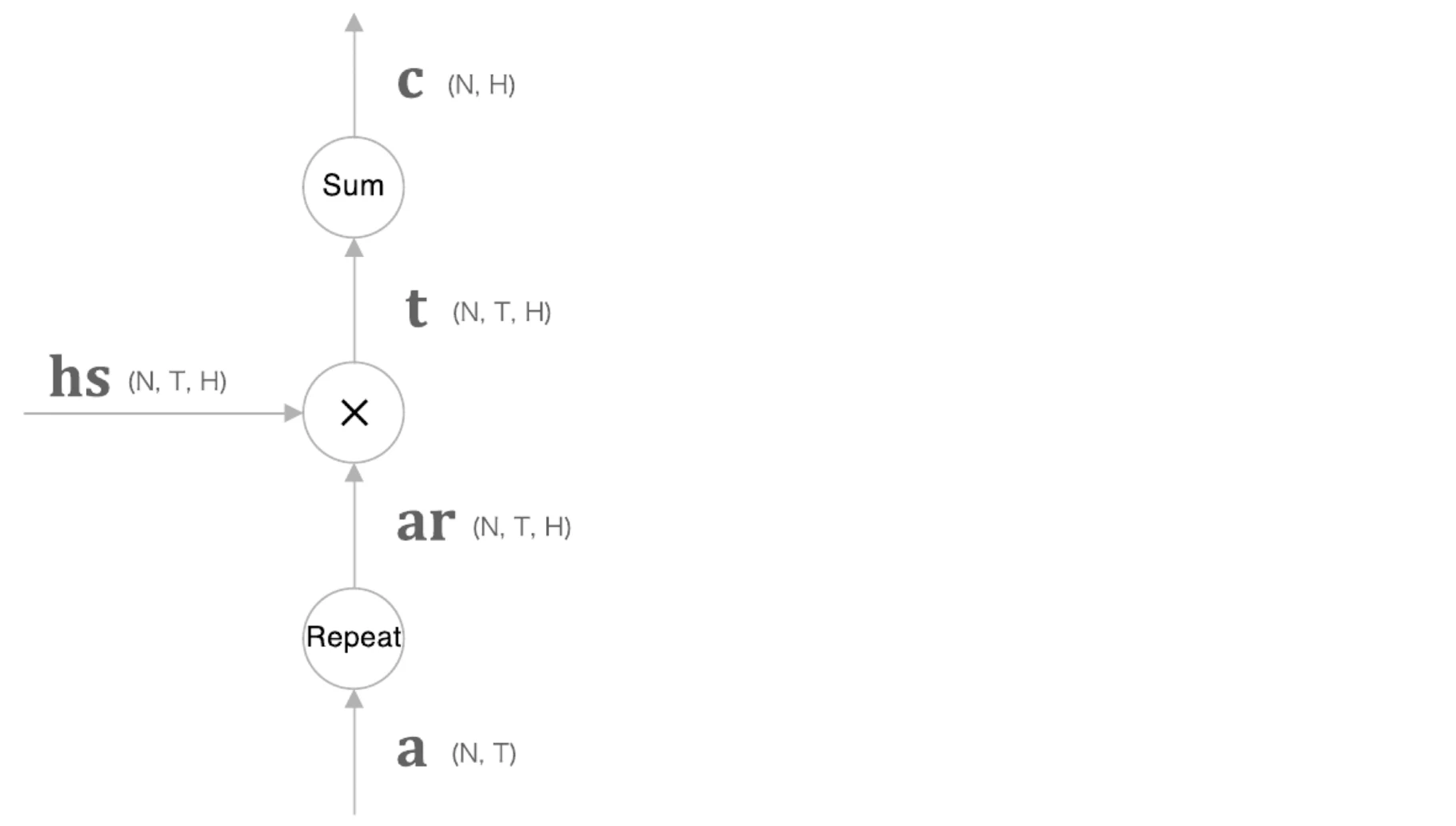
# (4,)

여기서 a는 각 시점의 중요도를 나타내는 attention weight이다.

a.reshape(5, 1).repeat(4, axis=1)을 통해 a를 hs와 같은 형상으로 확장한다.

그 다음 hs * ar로 원소별 곱을 수행하고, 시간축 방향으로 합을 구하면 context vector c가 된다.

이때 repeat(4, axis=1)은 계산 그래프에서 Repeat 노드에 해당한다.

따라서 역전파 시에는 미분의 선형성을 이용해 반복된 gradient를 다시 합치는 방식으로 처리한다.

가중합 계산은 행렬곱 matmul(a, hs)를 사용하는 것이 가장 간단해 보일 수 있다.

하지만 미니배치로 확장하면 형상 처리가 복잡해진다.

따라서 직관을 설명할 때는 repeat 기반 예제가 이해하기 쉽고, 실제 구현에서는 broadcasting, tensordot, einsum 등을 사용할 수 있다.

미니배치 가중합 계산

미니배치까지 고려하면 hs의 형상은 다음과 같다.

$$\mathrm{hs} \in \mathbb{R}^{N \times T \times H}$$

여기서 각 기호는 다음 의미이다.

• $N$: 미니배치 크기이다.
• $T$: 시계열 길이이다.
• $H$: hidden state 차원이다.

attention weight a의 형상은 다음과 같다.

$$a \in \mathbb{R}^{N \times T}$$

미니배치 가중합 계산은 다음과 같이 구현할 수 있다.

N, T, H = 10, 5, 4
hs = np.random.randn(N, T, H)
a = np.random.randn(N, T)

ar = a.reshape(N, T, 1).repeat(H, axis=2)

t = hs * ar
print(t.shape)
# (10, 5, 4)

c = np.sum(t, axis=1)
print(c.shape)
# (10, 4)

만약 x.shape = (X, Y, Z)라면 np.sum(x, axis=1).shape = (X, Z)이다.

즉 axis로 지정한 축이 합쳐지면서 사라진다.

여기서는 시간축 $T$ 방향으로 합을 구하므로, 최종 context vector c는 (N, H) 형상이 된다.

WeightSum 계층

가중합을 계층으로 구현하면 다음과 같다.

class WeightSum:
    def __init__(self):
        self.params, self.grads = [], []
        self.cache = None

    def forward(self, hs, a):
        N, T, H = hs.shape

        ar = a.reshape(N, T, 1)
        t = hs * ar
        c = np.sum(t, axis=1)

        self.cache = (hs, ar)
        return c

forward()에서는 attention weight a를 (N, T, 1)로 reshape한 뒤, hs와 곱한다.

이때 NumPy broadcasting에 의해 ar이 hidden dimension 방향으로 확장되어 계산된다.

그 다음 시간축 axis=1 방향으로 합을 구해 context vector c를 만든다.

역전파는 다음과 같다.

    def backward(self, dc):
        hs, ar = self.cache
        N, T, H = hs.shape
        dt = dc.reshape(N, 1, H).repeat(T, axis=1)
        dar = dt * hs
        dhs = dt * ar
        da = np.sum(dar, axis=2)

        return dhs, da

각 줄의 의미는 다음과 같다.

• dt = dc.reshape(N, 1, H).repeat(T, axis=1): sum 노드의 역전파이다.
• dar = dt * hs: 곱셈 노드에서 ar 쪽으로 흐르는 gradient이다.
• dhs = dt * ar: 곱셈 노드에서 hs 쪽으로 흐르는 gradient이다.
• da = np.sum(dar, axis=2): repeat 또는 broadcasting으로 확장된 차원을 다시 합치는 역전파이다.

수식으로 정리하면 다음과 같다.

$$\begin{aligned} &\text{입력: } \mathrm{dc} \in \mathbb{R}^{N \times H} \\ &\mathrm{hs}, \mathrm{ar} = \text{cache} \quad (\mathrm{hs} \in \mathbb{R}^{N \times T \times H},\ \mathrm{ar} \in \mathbb{R}^{N \times T \times H}) \\ &dt = \text{repeat}(\mathrm{dc}, T, \text{axis}=1) \in \mathbb{R}^{N \times T \times H} \\ &dar = dt \odot \mathrm{hs} \\ &dhs = dt \odot \mathrm{ar} \\ &da = \sum_{k=1}^{H} dar_{:, :, k} \in \mathbb{R}^{N \times T} \\ &\text{출력: } dhs, da \end{aligned}$$

Decoder 개선 2: Attention Weight 계산

Attention에서는 가중치 a를 통해 context vector c를 계산한다.

이때 a도 사람이 직접 정하는 것이 아니라 데이터로부터 자동으로 학습된다.

각 단어의 가중치 a를 구하는 방법 중 하나는 dot product 기반 score를 사용하는 것이다.

Encoder hidden states hs의 각 행과 Decoder의 현재 hidden state h 사이의 유사도를 내적으로 계산한다.

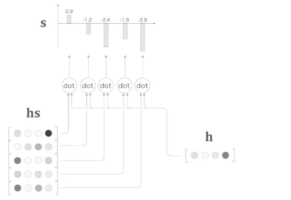
여기서 s는 softmax 적용 전의 유사도 score이다.

이 score에 softmax를 적용하면 attention weight a가 된다.

$$a = \mathrm{softmax}(s)$$

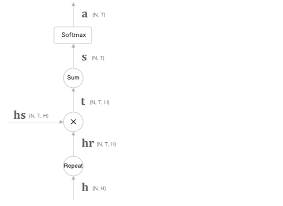
미니배치로 처리하는 예시는 다음과 같다.

N, T, H = 10, 5, 4
hs = np.random.randn(N, T, H)
h = np.random.randn(N, H)
hr = h.reshape(N, 1, H).repeat(T, axis=1)

t = hs * hr
print(t.shape)
# (10, 5, 4)

s = np.sum(t, axis=2)
print(s.shape)
# (10, 5)

softmax = Softmax()
a = softmax.forward(s)
print(a.shape)
# (10, 5)

hs와 hr을 원소별 곱한 뒤 마지막 차원 $H$를 따라 합을 취하면, 두 벡터의 내적을 배치 $N$과 시퀀스 길이 $T$마다 구한 형태가 된다.

즉 s는 각 입력 시점의 hidden state가 현재 Decoder hidden state h와 얼마나 비슷한지를 나타내는 score이다.

Attention Weight의 계산 그래프는 다음과 같다.

AttentionWeight 계층

Attention weight를 계층으로 구현하면 다음과 같다.

class AttentionWeight:
    def __init__(self):
        self.params, self.grads = [], []
        self.softmax = Softmax()
        self.cache = None

    def forward(self, hs, h):
        N, T, H = hs.shape

        hr = h.reshape(N, 1, H)
        t = hs * hr
        s = np.sum(t, axis=2)
        a = self.softmax.forward(s)

        self.cache = (hs, hr)
        return a

    def backward(self, da):
        hs, hr = self.cache
        N, T, H = hs.shape

        ds = self.softmax.backward(da)
        dt = ds.reshape(N, T, 1).repeat(H, axis=2)
        dhs = dt * hr
        dhr = dt * hs
        dh = np.sum(dhr, axis=1)

        return dhs, dh

forward()에서는 hs와 h의 내적 score를 구한 뒤, softmax를 통과시켜 attention weight a를 만든다.

backward()에서는 softmax의 역전파를 먼저 수행하고, 내적 계산을 구성했던 원소별 곱과 sum 연산을 거꾸로 따라간다.

최종적으로 Encoder hidden states 쪽 gradient dhs와 Decoder 현재 hidden state 쪽 gradient dh를 반환한다.

Decoder 개선 3: Attention 계층

Attention 계층은 AttentionWeight 계층과 WeightSum 계층을 결합한 것이다.

먼저 AttentionWeight로 attention weight a를 구한다.

그 다음 WeightSum으로 hs와 a의 가중합을 계산해 context vector c를 만든다.

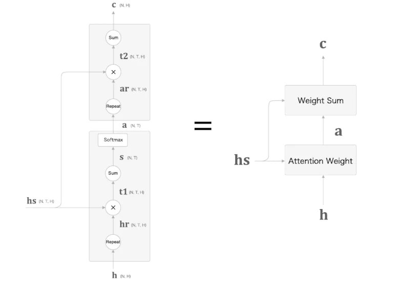
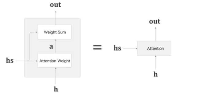
정리하면 다음과 같다.

Attention
= AttentionWeight
+ WeightSum

즉 Attention은 가중치 벡터를 생성하고, 그 가중치로 Encoder hidden states를 가중합하여 context vector를 만드는 계층이다.

Attention 계층 구현

class Attention:
    def __init__(self):
        self.params, self.grads = [], []
        self.attention_weight_layer = AttentionWeight()
        self.weight_sum_layer = WeightSum()
        self.attention_weight = None

    def forward(self, hs, h):
        a = self.attention_weight_layer.forward(hs, h)
        out = self.weight_sum_layer.forward(hs, a)
        self.attention_weight = a
        return out

    def backward(self, dout):
        dhs0, da = self.weight_sum_layer.backward(dout)
        dhs1, dh = self.attention_weight_layer.backward(da)
        dhs = dhs0 + dhs1
        return dhs, dh

Attention.forward()의 입력은 Encoder의 전체 hidden states hs와 Decoder의 현재 hidden state h이다.

출력은 context vector이다.

역전파에서는 두 경로에서 hs에 대한 gradient가 발생한다.

하나는 WeightSum에서 직접 흘러온 dhs0이고, 다른 하나는 AttentionWeight에서 score 계산을 통해 흘러온 dhs1이다.

따라서 두 gradient를 더해 최종 dhs를 만든다.

Attention이 추가된 Decoder

Attention은 Decoder의 LSTM과 Affine 계층 사이에 삽입된다.

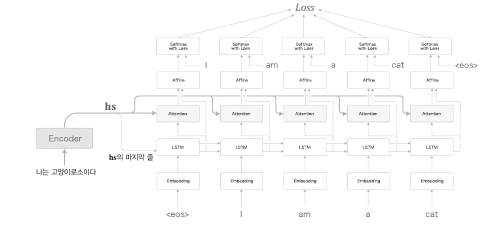
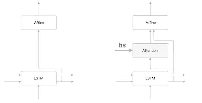
직관적으로 보면 Decoder에 Attention이 구한 context vector c의 정보를 추가하는 것이다.

즉 Affine 계층은 LSTM의 은닉 상태 벡터와 Attention 계층의 context vector를 함께 입력으로 받는다.

구현에서는 두 벡터를 연결한 벡터를 Affine 계층에 입력한다.

TimeAttention 구현

TimeAttention은 시계열 방향으로 펼쳐진 Attention 계층이다.

Decoder의 각 시점마다 Attention 계층을 하나씩 적용한다.

class TimeAttention:
    def __init__(self):
        self.params, self.grads = [], []
        self.layers = None
        self.attention_weights = None

    def forward(self, hs_enc, hs_dec):
        N, T, H = hs_dec.shape
        out = np.empty_like(hs_dec)
        self.layers = []
        self.attention_weights = []

        for t in range(T):
            layer = Attention()
            out[:, t, :] = layer.forward(hs_enc, hs_dec[:, t, :])
            self.layers.append(layer)
            self.attention_weights.append(layer.attention_weight)

        return out

    def backward(self, dout):
        N, T, H = dout.shape
        dhs_enc = 0
        dhs_dec = np.empty_like(dout)

        for t in range(T):
            layer = self.layers[t]
            dhs, dh = layer.backward(dout[:, t, :])
            dhs_enc += dhs
            dhs_dec[:, t, :] = dh

        return dhs_enc, dhs_dec

forward()에서는 Decoder의 각 시점 $t$마다 Attention 계층을 생성하고, hs_enc와 hs_dec[:, t, :]를 입력으로 넣는다.

backward()에서는 각 시점의 Attention 계층을 역전파한다.

Encoder hidden states hs_enc는 모든 Decoder 시점에서 참조되므로, 각 시점에서 나온 dhs를 누적한다.

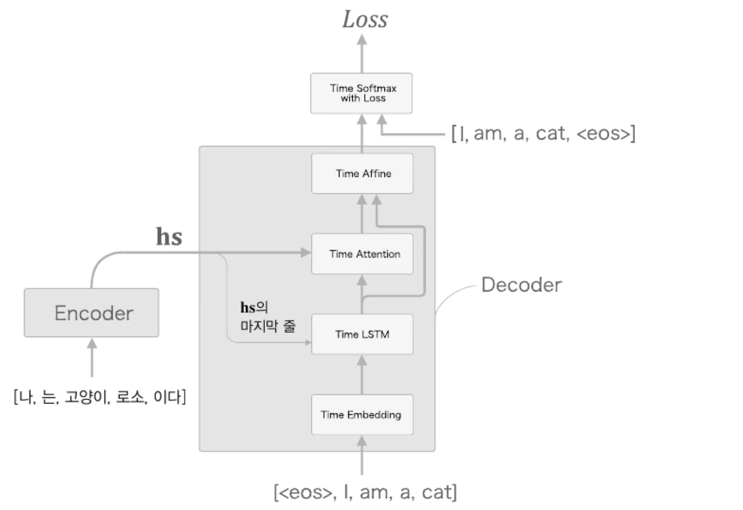
Attention을 갖춘 seq2seq

Attention을 갖춘 seq2seq는 크게 다음 구성요소로 이루어진다.

• AttentionEncoder
• AttentionDecoder
• AttentionSeq2seq

Encoder 쪽의 핵심 변화는 전체 hs를 넘겨주는 것이다.

기존 seq2seq에서는 마지막 hidden state만 중요하게 사용했지만, Attention 구조에서는 Decoder가 모든 Encoder hidden states를 참조해야 한다.

AttentionDecoder

Attention을 적용한 Decoder 구조는 다음과 같다.

AttentionDecoder에는 generate() 메서드도 포함된다.

class AttentionDecoder:
    def __init__(self, vocab_size, wordvec_size, hidden_size):
        V, D, H = vocab_size, wordvec_size, hidden_size
        rn = np.random.randn

        embed_W = (rn(V, D) / 100).astype('f')
        lstm_Wx = (rn(D, 4 * H) / np.sqrt(D)).astype('f')
        lstm_Wh = (rn(H, 4 * H) / np.sqrt(H)).astype('f')
        lstm_b = np.zeros(4 * H).astype('f')
        affine_W = (rn(2 * H, V) / np.sqrt(2 * H)).astype('f')
        affine_b = np.zeros(V).astype('f')

        self.embed = TimeEmbedding(embed_W)
        self.lstm = TimeLSTM(lstm_Wx, lstm_Wh, lstm_b, stateful=True)
        self.attention = TimeAttention()
        self.affine = TimeAffine(affine_W, affine_b)
        layers = [self.embed, self.lstm, self.attention, self.affine]

        self.params, self.grads = [], []
        for layer in layers:
            self.params += layer.params
            self.grads += layer.grads

    def forward(self, xs, enc_hs):
        h = enc_hs[:, -1]
        self.lstm.set_state(h)

        out = self.embed.forward(xs)
        dec_hs = self.lstm.forward(out)
        c = self.attention.forward(enc_hs, dec_hs)
        out = np.concatenate((c, dec_hs), axis=2)
        score = self.affine.forward(out)

        return score

    def backward(self, dscore):
        dout = self.affine.backward(dscore)
        N, T, H2 = dout.shape
        H = H2 // 2

        dc, ddec_hs0 = dout[:, :, :H], dout[:, :, H:]
        denc_hs, ddec_hs1 = self.attention.backward(dc)
        ddec_hs = ddec_hs0 + ddec_hs1
        dout = self.lstm.backward(ddec_hs)
        dh = self.lstm.dh
        denc_hs[:, -1] += dh
        self.embed.backward(dout)

        return denc_hs

    def generate(self, enc_hs, start_id, sample_size):
        sampled = []
        sample_id = start_id
        h = enc_hs[:, -1]
        self.lstm.set_state(h)

        for _ in range(sample_size):
            x = np.array([sample_id]).reshape((1, 1))

            out = self.embed.forward(x)
            dec_hs = self.lstm.forward(out)
            c = self.attention.forward(enc_hs, dec_hs)
            out = np.concatenate((c, dec_hs), axis=2)
            score = self.affine.forward(out)

            sample_id = np.argmax(score.flatten())
            sampled.append(sample_id)

        return sampled

forward()와 generate()에서는 TimeAttention의 출력 c와 LSTM 출력 dec_hs를 np.concatenate()로 연결하여 하나의 행렬로 전달한다.

Affine 계층의 입력 차원이 2 * H인 이유도 여기에 있다.

Attention context vector의 차원 $H$와 Decoder hidden state의 차원 $H$를 연결하므로 전체 차원은 $2H$가 된다.

AttentionSeq2seq

기존 seq2seq 구조에서 다음과 같이 구성요소를 바꾼다.

• Encoder를 AttentionEncoder로 바꾼다.
• Decoder를 AttentionDecoder로 바꾼다.

class AttentionSeq2seq(Seq2seq):
    def __init__(self, vocab_size, wordvec_size, hidden_size):
        args = vocab_size, wordvec_size, hidden_size
        self.encoder = AttentionEncoder(*args)
        self.decoder = AttentionDecoder(*args)
        self.softmax = TimeSoftmaxWithLoss()

        self.params = self.encoder.params + self.decoder.params
        self.grads = self.encoder.grads + self.decoder.grads

전체적으로 보면 Encoder는 모든 hidden states를 반환하고, Decoder는 각 시점마다 Attention을 통해 필요한 Encoder hidden state 정보를 참조한다.

Attention: 날짜 형식 변환 예제

예제 문제는 날짜가 들어오면 표준 날짜 형식으로 변환하는 것이다.

# coding: utf-8
import sys
sys.path.append('..')
sys.path.append('../ch07')
import numpy as np
import matplotlib.pyplot as plt
from dataset import sequence
from common.optimizer import Adam
from common.trainer import Trainer
from common.util import eval_seq2seq
from attention_seq2seq import AttentionSeq2seq
from ch07.seq2seq import Seq2seq
from ch07.peeky_seq2seq import PeekySeq2seq


# 데이터 읽기
(x_train, t_train), (x_test, t_test) = sequence.load_data('date.txt')
char_to_id, id_to_char = sequence.get_vocab()

# 입력 문장 반전
x_train, x_test = x_train[:, ::-1], x_test[:, ::-1]

# 하이퍼파라미터 설정
vocab_size = len(char_to_id)
wordvec_size = 16
hidden_size = 256
batch_size = 128
max_epoch = 10
max_grad = 5.0

model = AttentionSeq2seq(vocab_size, wordvec_size, hidden_size)
# model = Seq2seq(vocab_size, wordvec_size, hidden_size)
# model = PeekySeq2seq(vocab_size, wordvec_size, hidden_size)

optimizer = Adam()
trainer = Trainer(model, optimizer)

acc_list = []
for epoch in range(max_epoch):
    trainer.fit(x_train, t_train, max_epoch=1,
                batch_size=batch_size, max_grad=max_grad)

    correct_num = 0
    for i in range(len(x_test)):
        question, correct = x_test[[i]], t_test[[i]]
        verbose = i < 10
        correct_num += eval_seq2seq(model, question, correct,
                                    id_to_char, verbose, is_reverse=True)

    acc = float(correct_num) / len(x_test)
    acc_list.append(acc)
    print('정확도 %.3f%%' % (acc * 100))


model.save_params()

# 그래프 그리기
x = np.arange(len(acc_list))
plt.plot(x, acc_list, marker='o')
plt.xlabel('에폭')
plt.ylabel('정확도')
plt.ylim(-0.05, 1.05)
plt.show()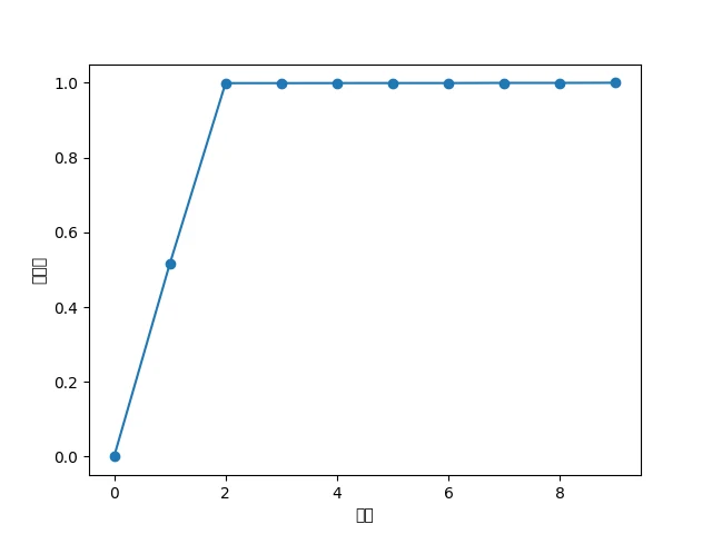

Attention 시각화

Attention은 학습된 alignment를 시각화할 수 있다는 장점도 있다.

가로축은 입력 문장이고, 세로축은 출력 문장이다.

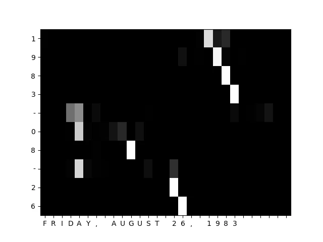
시각화 결과를 보면 Decoder가 각 출력 문자를 생성할 때 입력 문장의 어느 위치에 주목했는지 확인할 수 있다.

예를 들어 날짜 형식 변환 문제에서는 출력 위치가 입력 날짜의 특정 문자 위치와 대응된다.

Attention weight를 시각화하면 이 대응 관계가 어느 정도 자동으로 학습되었는지 볼 수 있다.